Interference edge filters are derived from the basic quarter-wave stack, characterized by a sharp transition between high-reflectance (low-transmission) and high-transmission regions, making them inherently suitable as shortwave or longwave-pass filters. However, the inherent ripple in the pass region must be reduced to create a useful edge filter, a task greatly simplified today by computer-aided design, though older analytical techniques remain valuable for theoretical understanding.
1. The Quarter-Wave Stack
The quarter-wave stack, a fundamental type of interference edge filter, produces alternating high-reflectance zones and high-transmission regions. The transmission curve of a typical stack is shown in Figure 7.2, demonstrating how the system can function as:
- A longwave-pass filter with an edge at 5.0 μm,
- A shortwave-pass filter with an edge at 3.3 μm.
These edge positions can be adjusted by changing the monitoring wavelength.

Applications and Limitations
In some cases, the rejection zone’s width is sufficient, such as when eliminating light in a narrow spectral region or when the detector is insensitive to wavelengths beyond the rejection zone. However, most applications require extending the rejection zone to block all wavelengths shorter or longer than a specific value. This can be achieved by:
- Adding additional filters to broaden the rejection zone.
- Combining absorption filters with interference filters:
- Absorption filters offer deep rejection but lack flexibility as their edge positions are fixed by material properties.
- Interference filters provide flexibility and can be deposited on absorption filters or made from materials with intrinsic absorption edges.
Ripple in the Pass Region
A significant challenge is the ripple in the pass region of the transmission curve, as seen in Figure 7.2. Ripple reduces filter performance and must be minimized. The cause of ripple is complex, involving intricate mathematical relationships.
Historical Insight
Epstein’s 1952 paper provided foundational methods to understand and address ripple, enabling predictions and improvements in filter performance. This insight is essential for designing interference edge filters with reduced ripple and extended functionality.
2. Symmetrical Multilayers and the Herpin Index
The concept of symmetrical multilayers, introduced in Epstein’s 1952 paper, revolutionized thin-film filter design by demonstrating the equivalence of a symmetrical combination of films to a single optical layer. This foundational concept has become a cornerstone of modern thin-film design.
Symmetrical Multilayers and Equivalent Layers
A thin-film arrangement is symmetrical if each half is a mirror image of the other. The simplest example is a three-layer structure, with a central layer sandwiched between identical outer layers. Such a structure, called a symmetrical period, can be mathematically treated as a single equivalent layer with:
- Phase thickness (\( \gamma \)),
- Equivalent admittance (\( E \), also known as the Herpin admittance).
If a multilayer consists of repeated symmetrical periods, the entire stack can be treated as a single layer with:
- Phase thickness = \( s\gamma \),
- Admittance = \( E \),
where \( s \) is the number of periods.
Characteristic Matrix for a Symmetrical Three-Layer Period
For a three-layer period \( pqp \), composed of dielectric materials without absorption, the characteristic matrix is derived as:
\[
M =
\begin{bmatrix}
M_{11} & M_{12} \\
M_{21} & M_{22}
\end{bmatrix},
\]
with:
- \( M_{11} = M_{22} = \cos\gamma \),
- \( M_{12} = iE\sin\gamma \),
- \( M_{21} = iE\sin\gamma \),
where:
\[
\gamma = \arccos(M_{11}),
\quad
E = \frac{M_{21}}{M_{12}}.
\]
These equations allow the symmetrical combination to be represented as a single equivalent layer.
Extension to Multilayers
This result extends to any symmetrical period, no matter the number of layers. By progressively replacing symmetrical sections with equivalent layers, a multilayer structure can be reduced to a single equivalent layer. This simplifies both analysis and visualization, as the multilayer properties are easier to interpret in terms of a single layer.
Stop Bands and Pass Bands
The symmetry leads to distinct stop bands (high reflectance) and pass bands (low reflectance with fringes):
- Stop bands occur when \( \gamma \) and \( E \) are imaginary, leading to reflectance approaching unity as the number of periods increases.
- Pass bands occur when \( \gamma \) and \( E \) are real, and the multilayer acts like a dielectric slab with increasingly dense fringes.
The edges of these bands are defined by \( M_{11} = -1 \), with \( \gamma \) and \( E \) computed using more detailed expressions derived from the matrix elements.
Simplifications for Quarter-Wave Stacks
For the specific case of a quarter-wave stack, these expressions simplify, making the analysis more tractable. The principles of symmetrical multilayers apply directly, allowing for efficient design and performance predictions.
3. Application of the Herpin Index to the Quarter-Wave Stack
The Herpin Index can be directly applied to quarter-wave stacks, with a minor adjustment to the design: adding a pair of eighth-wave layers at each end of the stack. These layers balance the structure, simplifying analysis and enhancing performance. Two typical configurations are:
1. High-Index Layers at Ends:
\[
H \quad LHLHLH \quad HLH
\]
Converts to:
\[
(H_2)L(H_2) \quad \dots \quad (H_2)L(H_2)
\]
2. Low-Index Layers at Ends:
\[
L \quad HLHLHL \quad LHL
\]
Converts to:
\[
(L_2)H(L_2) \quad \dots \quad (L_2)H(L_2)
\]
These configurations allow the use of symmetrical multilayer theory to calculate stop-band widths and pass-band performance effectively.
Stop-Band Width Calculation
The stop-band edges, determined by \( M_{11} = -1 \), are given by:
\[
\cos^2 \delta_p \cos^2 \delta_q – \frac{\sin^2 \delta_p \sin^2 \delta_q}{\eta_p \eta_q} = -1,
\]
where \( \delta \) is the optical phase thickness, and \( \eta \) represents admittances. Simplifying for quarter-wave stacks, where \( \delta = \frac{\pi}{2}g \) and \( g = \frac{\lambda_0}{\lambda} \), the stop-band width becomes:
\[
\Delta g = \frac{2}{\pi} \arcsin \left( \frac{\eta_q – \eta_p}{\eta_q + \eta_p} \right).
\]
This result matches earlier calculations and is maximized when the central layer is a quarter-wave and the outer layers are eighth-waves.
Equivalent Admittance in the Pass Band
The equivalent admittance (\( E \)) in the pass band, normalized by \( \eta_p \), is:
\[
\frac{E}{\eta_p} = \rho + \frac{1}{\rho} + (\rho – \frac{1}{\rho}) \cos 2\delta_q + \frac{2}{\rho} \sin 2\delta_q,
\]
where \( \rho = \frac{\eta_p}{\eta_q} \). This relationship holds for all symmetrical periods, including those with inhomogeneous layers.
Equivalent Phase Thickness
The equivalent phase thickness (\( \gamma \)) is calculated as:
\[
\gamma = \arccos \left( \cos^2 \delta_q – \frac{\sin^2 \delta_q}{\rho} \right).
\]
Near the high-reflectance zone edges, \( \gamma \) deviates significantly from the actual phase thickness. Elsewhere in the pass bands, \( \gamma \) closely matches the true thickness of the multilayer combination.
Visual Representation
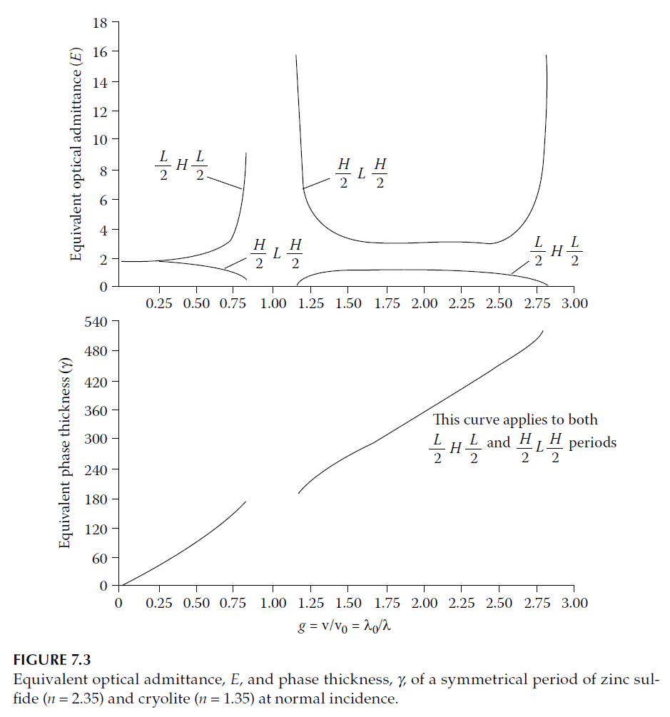
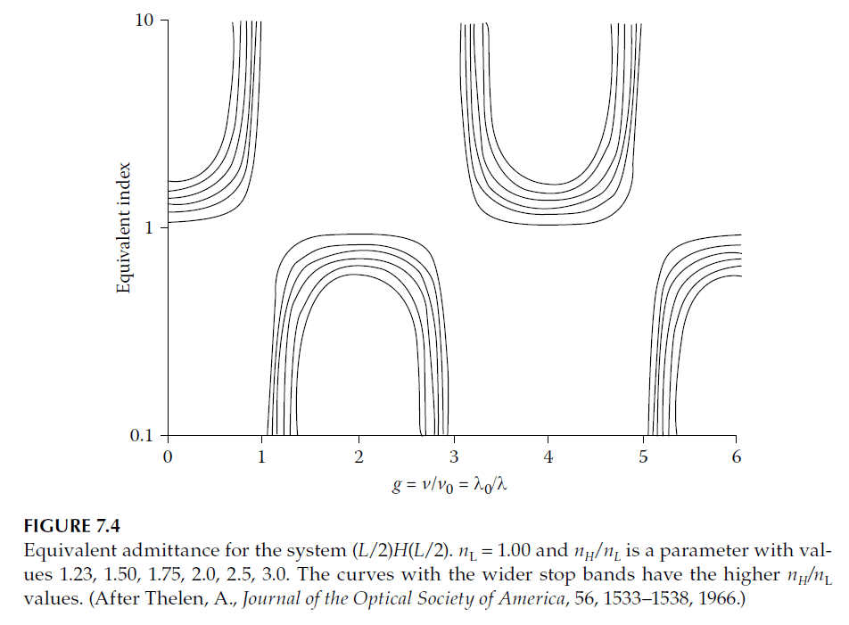
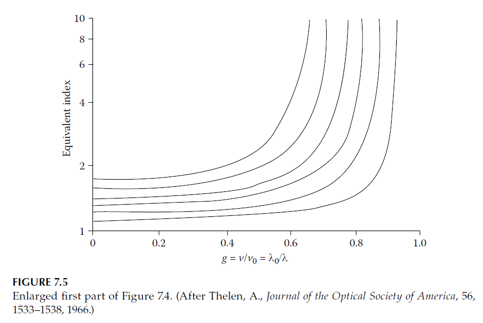
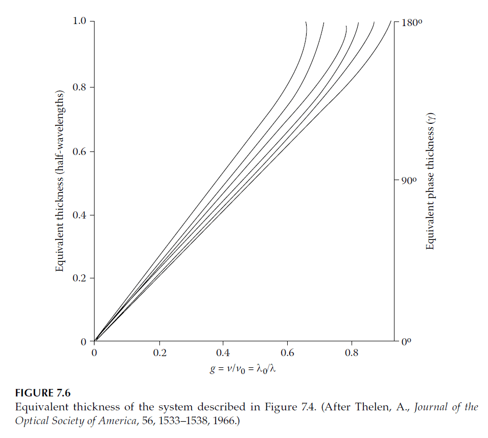
Figures 7.3–7.6, originally from Thelen’s work, illustrate:
- The equivalent admittance and phase thickness for zinc sulfide and cryolite combinations.
- Symmetrical relationships in optical parameters.
- How the equivalent phase thickness approximates the true thickness in pass bands but diverges at the high-reflectance zone edges.
These visualizations simplify interpreting the theoretical relationships and their dependence on material properties.
Practical Implications
Adding eighth-wave layers transforms quarter-wave stacks into symmetrical multilayers, making performance in the stop and pass bands calculable using Herpin Index theory. This approach, while analytical in origin, is complemented by modern computational methods for designing advanced thin-film filters.
4. Application of the Herpin Index to Multilayers Other Than Quarter-Waves
This section extends the application of the Herpin Index to multilayers where layer thicknesses deviate from the ideal eighth-wave | quarter-wave | eighth-wave configuration. Such variations significantly impact the equivalent admittance (\( E \)) and the reflectance zones of the multilayer.
General Behavior of Equivalent Admittance
When the relative thicknesses of layers are varied:
– For \( g \to 0 \):
The equivalent admittance (\( E \)) is confined within the range \( \eta_p \) and \( \eta_q \), where \( \eta_p \) and \( \eta_q \) are the optical admittances of the two materials.
\[
E \to \frac{\eta_p(1 + \psi \eta_q/\eta_p)}{1 + \psi \eta_p/\eta_q},
\]
where \( \psi = \frac{\sin 2\delta_q}{\sin 2\delta_p} \).
– For \( g \to 2 \):
At \( g = 2 \) (corresponding to \( 2\delta_p + \delta_q = 2\pi \)), the equivalent admittance becomes imaginary, signifying a zone of high reflectance. This occurs even when the theoretical condition predicts the multilayer should act as an absentee layer (as in an ideal configuration).
Reflection and Transmission Characteristics
1. Ideal Eighth-Wave | Quarter-Wave | Eighth-Wave Stacks:
- At \( g = 2 \), the multilayer ideally has no impact on the substrate reflectance, acting as an absentee layer due to the real admittance of the full-wave configuration.
- However, deviations from ideal thickness ratios introduce errors that result in a narrow high-reflectance zone, creating a half-wave hole in the transmission spectrum.
2. Impact of Thickness Deviations:
- When the layers are not precisely a half-wavelength thick, the absentee layer condition fails, leading to the emergence of high reflectance.
- The width of this spurious reflectance zone is narrow but significant, particularly in sensitive shortwave-pass filters.
Practical Considerations
The “half-wave hole” is a common issue in practical filter designs, especially in shortwave-pass filters. Its presence highlights the sensitivity of these designs to minor errors in layer thickness ratios. While theoretically predictable, eliminating these narrow reflectance dips requires precise control during fabrication.
5. Transmission at the Edge of a Stop Band
The level of transmission within the high-reflectance (stop band) region is a critical parameter of a filter. Thelen proposed a useful method for calculating the transmission at the edges of the band.
Let the multilayer consist of s fundamental periods, so its characteristic matrix is:
\[
[M_s] =
\begin{bmatrix}
\cos(s\gamma) & iE \sin(s\gamma) \\
\frac{i}{E} \sin(s\gamma) & \cos(s\gamma)
\end{bmatrix}
\]
At the stop band edges:
– \(\cos(s\gamma) \to 1\),
– \(\sin(s\gamma) \to 0\),
– \(E \to 0\) or \(E \to \infty\), depending on the specific layer combination.
For small \(\gamma\):
\[
\sin(s\gamma) \approx s\sin(\gamma),
\]
so the matrix simplifies to:
\[
[M_s] =
\begin{bmatrix}
1 & iEs\sin(\gamma) \\
\frac{i}{E}s\sin(\gamma) & 1
\end{bmatrix}.
\]
Depending on the configuration, either \(M_{12}\) or \(M_{21}\) approaches zero due to the determinant rule (\(M_{11}M_{22} – M_{12}M_{21} = 1\)). This results in one of two forms for the matrix:
\[
[M_s] =
\begin{bmatrix}
1 & 0 \\
0 & 1
\end{bmatrix},
\]
or
\[
[M_s] =
\begin{bmatrix}
0 & 1 \\
1 & 0
\end{bmatrix}.
\]
If \(\eta_0\) is the admittance of the incident medium and \(\eta_{\text{sub}}\) is the substrate’s admittance, the transmittance at the edge of the stop band is given by Equation 2.115:
\[
T = \frac{4\eta_0 \eta_{\text{sub}}}{|B + \eta_{\text{sub}}C|^2},
\]
where
\[
\begin{bmatrix}
B \\
C
\end{bmatrix}
=
[M_s]
\begin{bmatrix}
1 \\
\eta_0
\end{bmatrix}.
\]
Cases for \(M_{12} = 0\) or \(M_{21} = 0\)
1. If \(M_{12} = 0\):
\[
T = \frac{4\eta_0\eta_{\text{sub}}}{(\eta_0 + s\eta_{\text{sub}}|M_{21}|)^2}.
\]
2. If \(M_{21} = 0\):
\[
T = \frac{4\eta_0\eta_{\text{sub}}}{(\eta_0 + s\eta_{\text{sub}}|M_{12}|)^2}.
\]
Specific Case: Eighth-Wave | Quarter-Wave | Eighth-Wave Configuration
At the stop band edges:
\[
\cos^2(\delta_p) – \sin^2(\delta_p)\frac{\eta_q}{\eta_p} = -1,
\]
which simplifies to:
\[
\sin^2(\delta_p) = \frac{\eta_q(\eta_p – \eta_q)}{4\eta_p(\eta_p + \eta_q)}.
\]
Thus:
\[
M_{21} = \frac{\eta_q^2 – \eta_p^2}{\eta_p^2 + \eta_q^2},
\]
and:
\[
M_{12} = \frac{\eta_p^2 – \eta_q^2}{\eta_p^2 + \eta_q^2}.
\]
The above equations provide a robust framework for calculating transmittance at stop band edges. Depending on whether the equivalent admittance (\(E\)) is zero or infinite, either \(M_{12}\) or \(M_{21}\) becomes zero, guiding the appropriate substitution into the equations for transmittance. This method is particularly effective for analyzing layered structures like eighth-wave | quarter-wave | eighth-wave stacks, enabling precise performance predictions for optical filters.
6. Transmission in the Center of a Stop Band
For a simple quarter-wave stack, an expression for the transmittance at the center of the high-reflectance zone has already been derived. For the present multilayer configuration, which includes eighth-wave layers at the stack’s outer edges, the calculation becomes more complex. The stack structure can be represented as:
\[
p \, q \, p \, p \, q \, p \, p \, q \, p \ldots
\]
or equivalently:
\[
p \, q \, p \, q \, p \, q \ldots
\]
If there are \( s \) periods, the layer \( q \) appears \( s \) times. At the center of the high-reflectance zone, the matrix product becomes:
\[
[M] =
\begin{bmatrix}
0 & i\eta_q \\
i\eta_q & 0
\end{bmatrix}
\begin{bmatrix}
\eta_p & 0 \\
0 & \frac{1}{\eta_p}
\end{bmatrix}
\ldots
\]
By expanding and simplifying this expression, the resulting matrix becomes:
\[
[M] =
\begin{bmatrix}
0 & -i\eta_q^s \\
-i\eta_q^s & 0
\end{bmatrix}.
\]
Let \(\eta_{\text{sub}}\) be the substrate’s admittance. Then:
\[
\begin{bmatrix}
B \\
C
\end{bmatrix}
=
\begin{bmatrix}
1 – \frac{\eta_q^s}{\eta_p^s} \\
\eta_{\text{sub}} – \frac{\eta_p^s}{\eta_q^s}
\end{bmatrix}.
\]
The transmittance \(T\) is calculated using Equation 2.115:
\[
T = \frac{4\eta_0 \eta_{\text{sub}}}{|B + \eta_{\text{sub}}C|^2}.
\]
Substituting the values of \(B\) and \(C\) yields:
\[
T = \frac{16\eta_0 \eta_{\text{sub}}}{\Big((\eta_{\text{sub}} + \eta_q^s)(\eta_p^s + \eta_{\text{sub}}) – (\eta_p^s – \eta_q^s)^2\Big)^2}.
\]
Simplification for Large \(s\)
When \(s\) is sufficiently large, \(\eta_H^s\) and \(\eta_L^s\) dominate, leading to:
\[
T = \frac{16\eta_0 \eta_{\text{sub}}}{\Big(\eta_H \eta_L (\eta_H + \eta_L)\Big)^2},
\]
where \(\eta_p\) corresponds to either \(\eta_H\) or \(\eta_L\), depending on whether the stack terminates with a high- or low-index layer.
This final expression highlights the dependency of the transmittance at the center of the stop band on the layer refractive indices and the admittance of the substrate and incident medium. It serves as a useful formula for evaluating multilayer filter performance in this critical region.
7. Transmission in the Pass Band
In the pass band, a multilayer can be approximated as a single layer with slightly variable optical thickness and admittance. Consider the configuration \([(L/2)H(L/2)]^s\). Figure 7.7 illustrates the curve of the equivalent admittance \(E\) for the period \([(L/2)H(L/2)]\) and its equivalent phase thickness \(\gamma\).
Reflection Behavior of a Single Transparent Layer
For a real single transparent layer on a transparent substrate, the reflectance oscillates between two limits, depending on whether the optical thickness is equivalent to an integral number of quarter-waves:
1. Even number of quarter-waves (half-waves): The layer behaves as an absentee layer, and the reflectance equals that of the bare substrate:
\[
R_{\text{sub}} = \left(\frac{\eta_0 – \eta_{\text{sub}}}{\eta_0 + \eta_{\text{sub}}}\right)^2,
\]
where \(\eta_{\text{sub}}\) is the substrate’s admittance, and \(\eta_0\) is the incident medium’s admittance.
2. Odd number of quarter-waves: The reflectance depends on the film’s admittance \(\eta_f\) as:
\[
R_f = \left(\frac{\eta_0^2 – \eta_f\eta_{\text{sub}}}{\eta_0^2 + \eta_f\eta_{\text{sub}}}\right)^2.
\]
The maximum and minimum reflectance values form the envelopes of the reflectance curve, described by Equations 7.37 and 7.38:
\[
R_{\text{sub}} = \left(\frac{\eta_0 – \eta_{\text{sub}}}{\eta_0 + \eta_{\text{sub}}}\right)^2
\]
and
\[
R_f = \left(\frac{\eta_0^2 – E\eta_{\text{sub}}}{\eta_0^2 + E\eta_{\text{sub}}}\right)^2,
\]
where \(E\) is the equivalent admittance of the multilayer.
Wavelengths of Reflection Maxima and Minima
The actual wavelengths of maxima and minima occur at optical thicknesses \(D\) given by:
– For maxima: \(D = (2m+1)\lambda/4, m = 0, 1, 2, \ldots\)
– For minima: \(D = 2m\lambda/4, m = 1, 2, 3, \ldots\)
Multilayer Reflection in the Pass Band
For the multilayer, the reflectance oscillates between:
\[
R_{\text{sub}} = \left(\frac{\eta_0 – \eta_{\text{sub}}}{\eta_0 + \eta_{\text{sub}}}\right)^2
\]
and
\[
R_E = \left(\frac{\eta_0^2 – E\eta_{\text{sub}}}{\eta_0^2 + E\eta_{\text{sub}}}\right)^2,
\]
where \(E\) replaces \(\eta_f\) as the multilayer’s equivalent admittance. These correspond to even and odd multiples of \(\pi/2\) for the equivalent phase thickness \(s\gamma\), respectively:
\[
\gamma = \frac{m\pi}{2s}, \, m = 1, 3, 5, \ldots \, \text{(for maxima)},
\]
and
\[
\gamma = \frac{m\pi}{s}, \, m = 1, 2, 3, \ldots \, \text{(for minima)}.
\]
At the very edge of the pass band, where the equivalent phase thickness is \(\pi\), the multilayer should act as an absentee layer. However, due to the equivalent admittance being zero or infinite at this point, the multilayer cannot behave as a true absentee layer, and the previously derived expressions (7.26–7.36) must be applied.
Ripple in the Pass Band
The excessive ripple in the pass band is caused by mismatching between the equivalent admittance of the substrate, the multilayer stack, and the medium. To reduce the ripple, better matching of these admittances is necessary.
Figure 7.7 illustrates these principles using a four-period multilayer as an example. Importantly, the envelopes of the reflectance curve remain independent of the number of periods, emphasizing that ripple reduction depends on admittance matching rather than the number of layers.

8. Reduction of Pass-Band Ripple
Reducing ripple in the pass band can be achieved through several approaches:
1. Matching the Equivalent Admittance
The simplest method is to select a combination of materials whose equivalent admittance closely matches that of the substrate. This is effective if the bare substrate’s reflection loss is low. For instance:
- \([(H/2)L(H/2)]\) with \(\eta_H = 2.35\) and \(\eta_L = 1.35\) works well as a longwave-pass filter on glass (Figure 7.8).
- \([(L/2)H(L/2)]\) is more suitable for a shortwave-pass filter (also shown in Figure 7.8).
This method requires a low-index substrate, such as glass in the visible spectrum, but may not work well for high-index substrates like silicon or germanium in the infrared without modification.

2. Varying Film Thickness
Welford suggested varying the thicknesses of the layers in the basic period to adjust the equivalent admittance closer to the desired value. However, this method is rarely used and is limited by the substrate’s low reflection loss and index.
3. Adding Matching Layers
A common and effective method is to add quarter-wave matching layers to either side of the multilayer:
– A layer with admittance \(\eta_3\) is added between the multilayer and the substrate.
– A layer with admittance \(\eta_1\) is added between the multilayer and the incident medium.
Good matching is achieved when:
\[
\eta_1 = \sqrt{\eta_0 \eta_E}, \quad \eta_3 = \sqrt{\eta_E \eta_{\text{sub}}},
\]
where:
– \(\eta_0\): Admittance of the incident medium,
– \(\eta_E\): Equivalent admittance of the multilayer,
– \(\eta_{\text{sub}}\): Admittance of the substrate.
These layers act as antireflection coatings between the multilayer and its surroundings.
4. Performance Check
The effectiveness of matching layers can be quickly evaluated by considering the reflectance envelopes:
1. Quarter-Wave Behavior
When the multilayer behaves as a quarter-wave layer, the equivalent admittance is:
\[
Y_E = \frac{\eta_1^2 \eta_{\text{sub}}}{\eta_3^2}.
\]
The reflectance is:
\[
R = \left(\frac{\eta_0\eta_1^2 – \eta_{\text{sub}} \eta_3^2}{\eta_0\eta_1^2 + \eta_{\text{sub}} \eta_3^2}\right)^2,
\]
which becomes zero if:
\[
\eta_1^2 \eta_{\text{sub}} = \eta_0 \eta_3^2.
\]
2. Half-Wave Behavior
When the multilayer behaves as a half-wave layer, it becomes an absentee, and the reflectance is:
\[
R = \left(\frac{\eta_0 – \eta_{\text{sub}}}{\eta_0 + \eta_{\text{sub}}}\right)^2.
\]
These conditions confirm that matching is optimized when:
\[
\eta_1 = \sqrt{\eta_0 \eta_E}, \quad \eta_3 = \sqrt{\eta_E \eta_{\text{sub}}}.
\]
5. Example
Figure 7.9 illustrates a shortwave-pass filter’s performance before and after matching layers are added. The envelopes, based on quarter-wave matching layers, show the improved performance. Figure 7.10 presents the computed reflectance. The ripple slightly exceeds the envelope’s predictions as \(g > 1.25\), reflecting the limitations of the quarter-wave assumption for other \(g\)-values.
This section demonstrates how effective matching—through material selection, thickness variation, or adding matching layers—reduces pass-band ripple, ensuring optimal filter performance.


9. Summary of Design Procedure So Far
A systematic design procedure for edge filters has been developed as follows:
Step 1: Select Materials
Choose two materials with different refractive indices that are transparent in the desired transmission region. Use these materials to construct a multilayer in the form \([(L/2)H(L/2)]^s\) or \([(H/2)L(H/2)]^s\).
- High Index Ratio: Aim for a high ratio of refractive indices to maximize the rejection zone width and the rejection level for a given number of periods.
- Rejection Zone Width: Use Equation 7.15 and refer to Figure 6.7.
- Rejection Level: Determine rejection levels at the zone edges using Equations 7.26, 7.27, 7.31, and 7.32, and at the center using Equation 7.36.
Step 2: Calculate Equivalent Admittance
- Compute the equivalent admittance of the stack using:
- The design curves in Figure 7.5,
- Limiting values of \(E\) from Equations 7.19 and 7.20 to assist interpolation.
Step 3: Estimate Reflectance Envelopes
Using Equations 7.39 and 7.40, estimate the reflectance envelopes to predict ripple levels. If needed:
- Identify ripple peaks and troughs using the curves for \(\gamma\) in Figure 7.6 and the method in Section 7.2.3.4.
Step 4: Add Matching Layers (Optional)
If ripple is excessive, add quarter-wave matching layers:
- Place one layer with admittance \(\eta_1\) between the multilayer and the incident medium,
- Place another with admittance \(\eta_3\) between the multilayer and the substrate.
For effective matching, the admittances should be:
\[
\eta_1 = \sqrt{\eta_0 \eta_E}, \quad \eta_3 = \sqrt{\eta_E \eta_{\text{sub}}},
\]
where \(\eta_0\) is the incident medium’s admittance, \(\eta_E\) is the equivalent admittance, and \(\eta_{\text{sub}}\) is the substrate admittance.
If exact materials for matching layers are unavailable, compromises are necessary. Evaluate their effectiveness using Equations 7.42 and 7.44.
Example: Shortwave-Pass Filter Design
An example design using germanium and zinc sulfide on a germanium substrate is shown in Figures 7.9 and 7.10, illustrating the application of these principles.
Computer Assistance
Although this method is analytical and provides a deeper understanding, most practical designs rely on computer-based calculations for:
- Determining equivalent parameters,
- Simulating ripple performance.
This approach significantly reduces manual effort while ensuring precision and efficiency.
10. More Advanced Procedures for Eliminating Ripple
At the present time, probably the most common technique for eliminating ripple is computer refinement, which is dealt with in more detail later in this tutorial. Computers are unable to make use of terms like “improve,” “better,” or “worse.” They deal with numbers, and their logic is based on whether one number is greater or less than another.
For a computer to be able to improve a design, the assessment of any improvement has to be based on a number, changes in which correspond to what we would understand as an improvement or a deterioration in performance. Usually, but not always, a decreasing number is used to indicate improving performance. This number, called the figure of merit, represents the performance to the computer. It is calculated by a set of rules, called the function of merit, that reside in the computer.
The figure of merit is generally the expression in a single number of the difference between the current design performance and a desired or target performance. In the refinement process, the computer makes changes to a design in a process that gradually reduces the gap, as defined by the figure of merit, between the current design performance and target performance. The various refinement processes differ in the instructions followed by the computer in altering the design, but all aim to ensure convergence to as favorable a figure of merit as possible.
Introduction to Computer Refinement
Computer refinement was introduced into optical coating design by Baumeister [6], who programmed a computer to estimate the effects of slight changes in the thicknesses of the individual layers on a merit function representing the deviation of the performance of the coating from the ideal. An initial design, not too far from ideal, was adopted, and the thicknesses of the layers were modified successively to gradually improve the performance.
The optimum thickness of any one layer is not independent of the thicknesses of the other layers, so the changes in thickness at each iteration could not be large without running the risk of instability. Computer speed and capacity have increased considerably since Baumeister’s early work, but the essentials of the method are still the same. Rather than change the layers successively, it is now more usual to estimate changes to be made in all the adjustable layers simultaneously. These changes are then made, and the new figure of merit is computed. Further changes are then estimated, and the process repeated.
Refinement Techniques
If the function of merit is considered as a surface in \( (p+1) \)-dimensional space, with \( p \) independent variables being layer thicknesses, then a common method involves determining the direction of slope of the merit surface and then altering the layer thicknesses to move along it. An enormous number of different techniques exist, and comparisons of various methods have tended to show that there is no universal best technique.
Computer refinement is a very powerful design aid, but it can function only with an initial design. It then modifies the design to improve the performance. Less commonly, complete design synthesis is employed. This involves both refinement and a process for complicating the design when the refinement reaches an impasse, that is, a minimum merit figure that is still unsatisfactory. Synthesis was introduced in the 1960s by Dobrowolski. The use of both refinement and synthesis in design has grown in pace with improvements in and availability of computers.
Limitations of Computer Techniques
It is important to recognize that computer techniques cannot find designs that do not or cannot exist. They have no appreciation of feasibility and are restricted to the parameter space in which they operate. The existence of efficient refinement techniques does not make analytical methods obsolete. Analytical techniques remain invaluable for:
- 1. Determining the feasibility of a design
- 2. Avoiding unrealistic searches, and
- 3. Setting up initial designs for refinement.
Matching Layers
The first and obvious method for improving our edge filter designs is to improve the efficiency of the matching layers. In the chapter on antireflection coatings, many multilayer coatings were discussed that gave better performance than single-layer coatings. The ultimate performance was obtained with an inhomogeneous layer. Unfortunately, as seen previously, the major problem with inhomogeneous layers is the attainment of a refractive index less than about 1.35, which is required for matching to air.
Jacobsson explored the matching of a multilayer longwave-pass filter \( [(H/2)L(H/2)]_6 \), consisting of germanium (\( n = 4.0 \)) and silicon monoxide (\( n = 1.80 \)), to a germanium substrate. His work is shown in Figure 7.11. With an inhomogeneous layer varying from \( n = 4.0 \) at the substrate to \( n = 1.52 \) at the multilayer, performance almost identical to that of the multilayer on a glass substrate (\( n = 1.52 \)) was achieved.

Symmetrical Period Designs
Young and Cristal noted that symmetrical period designs could reduce ripple effectively. They proposed treating symmetrical periods as equivalent layers. Using microwave techniques, they designed a filter by replacing each layer with a symmetrical period, achieving excellent performance (Figures 7.12 and 7.13).


Electrical Analogy and Further Techniques
Seeley and Smith developed an electrical analogy method to optimize multilayer filters. Using principles from lumped electrical filters, they calculated layer thicknesses for specified refractive indices. The method enabled systematic design, especially for complex filters like Tchebyshev types, as shown in Figure 7.18.

Practical Considerations
The manufacture of edge filters or any optical coating is not straightforward. If the expected performance of a simple design cannot be achieved in manufacture, attempting more complex designs is futile until sources of error are eliminated.