1. Maxwell’s Equations and Plane Electromagnetic Waves
To begin addressing thin-film problems, we start by solving Maxwell’s equations in conjunction with the relevant material equations. In isotropic media, these equations are expressed as:
\[\text{curl} \, \mathbf{H} = \nabla \times \mathbf{H} = \mathbf{j} + \frac{\partial \mathbf{D}}{\partial t}\tag{2.1}\]
\[\text{curl} \, \mathbf{E} = \nabla \times \mathbf{E} = -\frac{\partial \mathbf{B}}{\partial t} \tag{2.2}\]
\[\text{div} \, \mathbf{D} = \nabla \cdot \mathbf{D} = \rho \tag{2.3}\]
\[\text{div} \, \mathbf{B} = \nabla \cdot \mathbf{B} = 0 \tag{2.4}\]
\[\mathbf{j} = \sigma \mathbf{E} \tag{2.5}\]
\[\mathbf{D} = \epsilon \mathbf{E} \tag{2.6}\]
\[\mathbf{B} = \mu \mathbf{H} \tag{2.7}\]
Here, bold symbols indicate vector quantities. In anisotropic media, these equations become significantly more complex because the parameters \(\sigma\), \(\epsilon\), and \(\mu\) are tensors rather than scalar values.
This tutorial employs the International System of Units (SI) as consistently as possible. Table 2.1 provides definitions of the variables in the above equations along with their corresponding SI units.

To extend the set of equations, we can incorporate the following relationships:
\[\epsilon = \epsilon_r \epsilon_0 \tag{2.8}\]
\[\mu = \mu_r \mu_0 \tag{2.9}\]
\[\epsilon_0 \mu_0 = \frac{1}{c^2} \tag{2.10}\]
Here, \(\epsilon_0\) and \(\mu_0\) are the permittivity and permeability of free space, respectively; \(\epsilon_r\) and \(\mu_r\) are the relative permittivity and permeability, respectively; and \(c\) is the speed of light in free space. These constants are fundamental to electromagnetic theory, and their values are summarized in Table 2.2.
In the usual case, the parameters in Equations (2.8) through (2.10) do not depend on either \(\mathbf{E}\) or \(\mathbf{H}\), meaning the behavior of the medium is linear.
The analysis presented here is intentionally brief and simplified for application to thin-film problems. Assuming there is no space charge (\(\rho = 0\)), we can simplify Equation (2.3):
\[\text{div} \, \mathbf{D} = \epsilon (\nabla \cdot \mathbf{E}) = 0 \tag{2.11}\]
From this, solving for \(\mathbf{E}\), we derive:
\[\nabla \times \nabla \times \mathbf{E} = \nabla (\nabla \cdot \mathbf{E}) – \nabla^2 \mathbf{E} = -\mu \frac{\partial^2 \mathbf{E}}{\partial t^2} – \mu \sigma \frac{\partial \mathbf{E}}{\partial t} \tag{2.12}\]
Simplifying further, we obtain:
\[\nabla^2 \mathbf{E} = \mu \epsilon \frac{\partial^2 \mathbf{E}}{\partial t^2} + \mu \sigma \frac{\partial \mathbf{E}}{\partial t} \tag{2.13}\]
This equation represents the wave equation for the electric field in a conductive medium, incorporating both propagation and damping terms due to the material’s conductivity.

A similar expression applies to \(\mathbf{H}\).
To solve Equation (2.13), we consider a solution in the form of a linearly polarized plane harmonic wave, often referred to as a plane-polarized wave. We represent this wave using a complex form, where the physical interpretation corresponds to either the real or imaginary part of the expression:
\[\mathbf{E} = \mathbf{E}_0 \exp[i\omega(t – z/v)] \tag{2.14}\]
This represents a wave propagating along the \(z\)-axis with velocity \(v\). Here, \(\mathbf{E}_0\) is the vector amplitude, and \(\omega\) is the angular frequency of the wave. Because the system is linear, \(\omega\) remains invariant as the wave propagates through media with different properties. The use of the complex form simplifies handling phase changes, as they can be incorporated directly into the complex amplitude.
By introducing a relative phase \(\phi\), Equation (2.14) becomes:
\[\mathbf{E} = \mathbf{E}_0 \exp[i\omega(t – z/v + \phi)] = \mathbf{E}_0 \exp(i\phi) \exp[i\omega(t – z/v)] \tag{2.15}\]
Here, \(\mathbf{E}_0 \exp(i\phi)\) is the complex vector amplitude, and the scalar complex amplitude is \(|\mathbf{E}_0| \exp(i\phi)\). This expression (2.15) includes a relative phase \(\phi\) compared to Equation (2.14), and it effectively replaces the real amplitude in (2.14) with the complex amplitude.
In Equation (2.14), the time variable is placed first, followed by the spatial variable within the argument of the exponential. This ordering is a convention; alternatively, the spatial variable could come first.
However, under this convention, reversing the wave’s direction is straightforward—changing the minus sign to a plus sign inverts the spatial direction of propagation. In contrast, the alternative convention could lead to confusion, as flipping the sign would invert the time axis rather than the spatial direction. We adhere to the convention in Equation (2.14) throughout this tutorial.
For Equation (2.14) to satisfy Equation (2.13), the following condition must hold:
\[\frac{\omega^2}{v^2} = \omega^2 \epsilon \mu – i\omega \mu \sigma \tag{2.16}\]
In a vacuum, where \(\sigma = 0\) and \(v = c\), this simplifies to:
\[c^2 = \frac{1}{\epsilon_0 \mu_0} \tag{2.17}\]
This equation confirms that the speed of light \(c\) in a vacuum is determined by the permittivity \(\epsilon_0\) and permeability \(\mu_0\) of free space.
By multiplying Equation (2.16) by Equation (2.17) and dividing by \(\omega^2\), we derive:
\[\frac{c^2}{v^2} = \epsilon_r \mu_r – i \frac{\mu_r \sigma}{\omega \epsilon_0} \tag{2.18}\]
The term \(\frac{c}{v}\) is a dimensionless property of the medium, which we define as \(N\):
\[N = \frac{c}{v} = n – i k \tag{2.19}\]
Here, \(N\) is the complex refractive index, where \(n\) is the real part of the refractive index (often referred to simply as the refractive index in ideal dielectrics) and \(k\) is the extinction coefficient, representing the medium’s absorptive properties.
From Equation (2.18), two possible solutions for \(N\) exist, but only the one with a positive value for \(n\) is physically valid. If all parameters in Equation (2.18) are real, the following relationships hold:
\[n^2 – k^2 = \epsilon_r \mu_r \tag{2.20}\]
\[2nk = \frac{\mu_r \sigma}{\omega \epsilon_0} \tag{2.21}\]
The wave described by Equation (2.14) can now be expressed using the complex refractive index:
\[\mathbf{E} = \mathbf{E}_0 \exp \left[ i\omega t – \frac{2\pi N}{\lambda} z \right] \tag{2.22}\]
where \(\lambda = \frac{2\pi c}{\omega}\) is the wavelength in free space. Substituting \(N = n – ik\) into Equation (2.22) gives:
\[\mathbf{E} = \mathbf{E}_0 \exp\left(-\frac{2\pi k}{\lambda}z\right) \exp\left[i\omega t – \frac{2\pi n}{\lambda}z\right] \tag{2.23}\]
The term \(\exp\left(-\frac{2\pi k}{\lambda}z\right)\) represents the exponential decay of the wave’s amplitude due to absorption in the medium. The distance over which the amplitude decreases to \(1/e\) of its initial value is:
\[\frac{\lambda}{2\pi k}\]
This distance is called the absorption length.
The phase change produced by traveling a distance \(z\) in a medium with refractive index \(n\) is equivalent to the phase change produced by traveling a distance \(nz\) in a vacuum. This equivalent distance, \(nz\), is known as the optical distance. It differs from the physical distance (or geometrical distance) and is often more relevant in thin-film optics.
In thin-film applications, optical distances and thicknesses are critical because they directly influence interference patterns and other optical effects. As a result, optical properties often take precedence over purely geometrical considerations.
Since \(\mathbf{E}\) is constant, Equation (2.18) represents a linearly polarized plane wave propagating along the \(z\)-axis. For a similar wave propagating in an arbitrary direction defined by the directional cosines \((\alpha, \beta, \gamma)\), the expression becomes:
\[\mathbf{E} = \mathbf{E}_0 \exp\left[i\omega t – \frac{2\pi N}{\lambda} (\alpha x + \beta y + \gamma z)\right] \tag{2.24}\]
This represents the simplest form of a wave in an absorbing medium. In cases involving multiple absorbing thin films, a more complex wave expression may occasionally be required.
The direction of wave propagation is described by the unit vector \(\hat{s}\), defined as:
\[\hat{s} = \alpha \mathbf{i} + \beta \mathbf{j} + \gamma \mathbf{k}\]
where \(\mathbf{i}, \mathbf{j}, \mathbf{k}\) are unit vectors along the \(x\)-, \(y\)-, and \(z\)-axes, respectively.
From Equation (2.24), the time derivative of \(\mathbf{E}\) is:
\[\frac{\partial \mathbf{E}}{\partial t} = i\omega \mathbf{E}\]
Using Maxwell’s equations (Equations 2.1, 2.5, and 2.6), we have:
\[\text{curl} \, \mathbf{H} = \mathbf{j} + \epsilon \frac{\partial \mathbf{E}}{\partial t} = \sigma \mathbf{E} + \epsilon \frac{\partial \mathbf{E}}{\partial t} = \left(\sigma + i\omega \epsilon \right) \mathbf{E} = \frac{i\omega \epsilon N^2}{c^2} \mathbf{E}\]
For the curl operator, we express:
\[\text{curl} = \mathbf{i} \frac{\partial}{\partial x} + \mathbf{j} \frac{\partial}{\partial y} + \mathbf{k} \frac{\partial}{\partial z}\]
Using the wave’s propagation properties:
\[\frac{\partial}{\partial x} = -\frac{2\pi i N}{\lambda} \alpha, \quad \frac{\partial}{\partial y} = -\frac{2\pi i N}{\lambda} \beta, \quad \frac{\partial}{\partial z} = -\frac{2\pi i N}{\lambda} \gamma\]
Thus, we obtain:
\[\text{curl} \, \mathbf{H} = -i\omega N (\hat{s} \times \mathbf{H})\]
Substituting this into Maxwell’s equations yields:
\[-i\omega N (\hat{s} \times \mathbf{H}) = \frac{i\omega \epsilon N^2}{c^2} \mathbf{E}\]
Simplifying:
\[\hat{s} \times \mathbf{H} = -\frac{\mathbf{E}}{N c \mu} \tag{2.25}\]
Similarly, for the relationship between \(\mathbf{E}\) and \(\mathbf{H}\):
\[\hat{s} \times \mathbf{E} = \frac{\mathbf{H}}{N c \mu} \tag{2.26}\]
For this type of wave, \(\mathbf{E}\), \(\mathbf{H}\), and \(\hat{s}\) are mutually perpendicular and form a right-handed coordinate system. The term \(N/c\mu\) represents the characteristic optical admittance of the medium, denoted as \(y\). In free space, the optical admittance is given by:
\[Y = \sqrt{\frac{\epsilon_0}{\mu_0}} \approx 2.6544 \times 10^{-3} \, \text{S} \tag{2.27}\]
In a medium, the permeability is given by:
\[\mu = \mu_r \mu_0 \tag{2.28}\]
At optical frequencies, direct magnetic interactions are negligible, so \(\mu_r \approx 1\). Thus, the characteristic optical admittance \(y\) can be written as:
\[y = N Y \tag{2.29}\]
Finally, the magnetic field \(\mathbf{H}\) is related to \(\mathbf{E}\) through:
\[\mathbf{H} = y (\hat{s} \times \mathbf{E}) = N Y (\hat{s} \times \mathbf{E}) \tag{2.30}\]
1.1 The Poynting Vector
A critical feature of electromagnetic radiation is that it serves as a form of energy transport. The energy carried by the wave is typically what is observed. The instantaneous rate of energy flow per unit area is described by the Poynting vector:
\[\mathbf{S} = \mathbf{E} \times \mathbf{H} \tag{2.31}\]
The direction of \(\mathbf{S}\) indicates the direction of energy flow.
When dealing with complex numbers, linear operations—such as addition, subtraction, or multiplication by a real number—keep the real and imaginary parts independent. This allows us to use the complex representation of a wave in interference calculations, where waves are added or subtracted. The complex form offers significant advantages in these cases.
However, nonlinear operations, such as multiplying two complex numbers, mix their real and imaginary parts in the result. This poses a problem for directly using the complex form of the wave in certain calculations, such as the Poynting vector, since \(\mathbf{E}\) and \(\mathbf{H}\) are multiplied.
To address this issue, we must work with either the real or imaginary parts of the wave expressions. Using the real sine or cosine forms of the wave implies that the instantaneous Poynting vector oscillates at twice the frequency of the wave. For practical purposes, we focus on the mean value of the Poynting vector, which corresponds to the energy flow observed in measurements. This mean value is defined as the irradiance.
In the SI system, irradiance is measured in watts per square meter (\(\text{W·m}^{-2}\)). However, a challenge arises with notation: the SI symbol for irradiance is \(E\), which can easily be confused with the electric field strength, also denoted by \(E\). To avoid ambiguity, we adopt the symbol \(I\) for irradiance, even though this conflicts with the SI symbol for intensity.
The mean value of the Poynting vector, or irradiance, can be derived using the complex form of the wave without requiring explicit integration over a cycle. For a harmonic wave:
\[\mathbf{I} = \frac{1}{2} \text{Re}(\mathbf{E} \times \mathbf{H}^*) \tag{2.32}\]
Here, the asterisk (\(^*\)) denotes the complex conjugate, and \(\text{Re}\) represents the real part. The complex form must be used in this equation. The resulting \(\mathbf{I}\) is a vector quantity with the same direction as the wave’s energy flow.
The scalar irradiance, which is more commonly used, is simply the magnitude of the vector \(\mathbf{I}\). Because \(\mathbf{E}\) and \(\mathbf{H}\) are perpendicular, Equation (2.32) simplifies to:
\[I = \frac{1}{2} \text{Re}(E H^*) \tag{2.33}\]
where \(E\) and \(H\) are the scalar magnitudes of the electric and magnetic fields, respectively.
To calculate the net irradiance, the electric and magnetic fields (\(\mathbf{E}\) and \(\mathbf{H}\)) in Equation (2.32) must represent the total resultant fields from all the waves involved. This requirement is inherent in the derivation of the Poynting vector. The importance of this will become apparent in discussions of reflectance and transmittance, where multiple waves interact.
For a single, homogeneous, harmonic wave of the form given in Equation (2.24), the magnetic field \(\mathbf{H}\) is related to the electric field \(\mathbf{E}\) by:
\[\mathbf{H} = y (\hat{s} \times \mathbf{E})\]
Substituting this into the expression for the Poynting vector and applying Equation (2.32), we find the irradiance:
\[I = \frac{1}{2} Y n |\mathbf{E}|^2 \exp\left[-\frac{4\pi k}{\lambda} (\alpha x + \beta y + \gamma z)\right] \tag{2.34}\]
where \(Y\) is the characteristic admittance of free space, \(n\) is the real part of the refractive index, and \(k\) is the extinction coefficient. The term \((\alpha x + \beta y + \gamma z)\) represents the distance along the wave’s direction of propagation.
From Equation (2.24), the electric field magnitude is:
\[|\mathbf{E}| = |\mathbf{E}_0| \exp\left[-\frac{2\pi k}{\lambda} (\alpha x + \beta y + \gamma z)\right]\]
The product of \(\mathbf{E}\) and its complex conjugate \(\mathbf{E}^*\) yields:
\[|\mathbf{E}|^2 = |\mathbf{E}_0|^2 \exp\left[-\frac{4\pi k}{\lambda} (\alpha x + \beta y + \gamma z)\right]\]
Thus, the irradiance becomes:
\[I = \frac{1}{2} Y n |\mathbf{E}_0|^2 \exp\left[-\frac{4\pi k}{\lambda} (\alpha x + \beta y + \gamma z)\right] \tag{2.35}\]
The term \((\alpha x + \beta y + \gamma z)\) corresponds to the distance traveled along the direction of propagation. The irradiance decreases to \(1/e\) of its initial value after traveling a distance:
\[d = \frac{\lambda}{4\pi k}\]
The inverse of this distance defines the absorption coefficient \(\alpha\), given by:
\[\alpha = \frac{4\pi k}{\lambda} \tag{2.36}\]
It is important to note that this \(\alpha\) should not be confused with the direction cosine \(\alpha\).
The amplitude of the electric field at a point \((x, y, z)\) is:
\[|\mathbf{E}| = |\mathbf{E}_0| \exp\left[-\frac{2\pi k}{\lambda} (\alpha x + \beta y + \gamma z)\right]\]
This allows for a simpler expression for irradiance:
\[I = \frac{1}{2} Y n (\text{amplitude})^2 \tag{2.37}\]
or, in proportionality form:
\[I \propto n \cdot (\text{amplitude})^2 \tag{2.38}\]
This expression emphasizes the necessity of including the refractive index \(n\) when comparing irradiances. The more common approximation:
\[I \propto (\text{amplitude})^2 \tag{2.39}\]
is less accurate. When waves propagate through media of different refractive indices, neglecting \(n\) introduces significant errors. Thus, for precise calculations of reflectance, transmittance, and other optical properties, \(n\) must be incorporated as shown above.
2. The Simple Boundary
Thin-film filters usually consist of a number of boundaries between various homogeneous media, and it is the effect of these boundaries on an incident wave that we will wish to calculate. A single boundary is the simplest case.
First, we consider absorption-free media, i.e., \( k = 0 \). The arrangement is sketched in **Figure 2.1**. A plane harmonic wave is incident on a plane surface separating the incident medium from a second, or emergent, medium. The plane containing the normal to the surface and the direction of propagation of the incident wave is known as the **plane of incidence**, and the sketch corresponds to this plane.
We take the \( z \)-axis as the normal into the surface in the sense of the incident wave and the \( x \)-axis as normal to it and also in the plane of incidence. At a boundary, the tangential components of \( \mathbf{E} \) and \( \mathbf{H} \)—that is, the components along the boundary—are continuous across it because there is no mechanism that will change them. This boundary condition is fundamental in our thin-film theory.
The first problem we have is that the boundary conditions are incompatible with a simple traversal of the boundary by the incident wave. The discontinuity in the characteristic admittance implies a power discontinuity impossible in a simple boundary. This problem is immediately solved by introducing a reflected wave in the incident medium, and this, of course, is directly in line with our experience.
Our objective then becomes the calculation of the relative parameters of the three waves: incident, reflected, and transmitted. However, this introduces a further complication. We will use the boundary conditions to set up a set of equations from which we will extract the required relations.
The complication is that the reflected wave will certainly be traveling in a different sense from the others so that there will be differences in the phase factors that will considerably complicate the calculations. We can help ourselves enormously by defining the boundary by \( z = 0 \), eliminating the \( z \)-term from the phase factors at the boundary. Then the tangential components must be continuous for all values of \( x, y, \) and \( t \).
We therefore have three harmonic waves: an incident, a reflected, and a transmitted wave. Let the direction cosines of the unit vectors of the transmitted and reflected waves be given by \( (\alpha_t, \beta_t, \gamma_t) \) and \( (\alpha_r, \beta_r, \gamma_r) \), respectively. We already know the direction of the incident wave. We can therefore write the phase factors in the form:
**Incident wave:**
\[\exp\{i[\omega t – (2\pi n_0 / \lambda_i)(x \sin \vartheta_0 + z \cos \vartheta_0)]\}\]
**Reflected wave:**
\[\exp\{i[\omega t – (2\pi n_0 / \lambda_r)(\alpha_r x + \beta_r y + \gamma_r z)]\}\]
**Transmitted wave:**
\[\exp\{i[\omega t – (2\pi n_1 / \lambda_t)(\alpha_t x + \beta_t y + \gamma_t z)]\}\]
The relative phases of these waves are included in the complex amplitudes. For waves with these phase factors to satisfy the boundary conditions for all \( x, y, t \) at \( z = 0 \), the coefficients of these variables must be separately identically equal. Had we not already known that there would be no change in frequency, this would have confirmed it. Because the frequencies are constant, so, too, will be the free-space wavelengths.
Next:
\[0 \equiv n_0 \beta_r \equiv n_1 \beta_t\tag{2.39}\]
That is, the directions of the reflected and transmitted (or refracted) beams are confined to the plane of incidence. This, in turn, means that the direction cosines of the reflected and transmitted waves are of the form:
\[\alpha = \sin \vartheta, \quad \gamma = \cos \vartheta\tag{2.40}\]
Also:
\[n_0 \sin \vartheta_0 \equiv n_0 \alpha_r \equiv n_1 \alpha_t\]
so that if the angles of reflection and refraction are \( \vartheta_r \) and \( \vartheta_t \), respectively, then:
\[\vartheta_0 = \vartheta_r\tag{2.41}\]
That is, the angle of reflection equals the angle of incidence, and:
\[n_0 \sin \vartheta_0 = n_1 \sin \vartheta_t\]
The result appears more symmetrical if we replace \( \vartheta_t \) by \( \vartheta_1 \), giving:
\[n_0 \sin \vartheta_0 = n_1 \sin \vartheta_1\tag{2.42}\]
This is the familiar relationship known as **Snell’s law**. \( \gamma_r \) and \( \gamma_t \) are then given either by Equation (2.40) or by:
\[\alpha_r^2 + \gamma_r^2 = 1 \quad \text{and} \quad \alpha_t^2 + \gamma_t^2 = 1\tag{2.43}\]
Note that for the reflected beam, we must choose the negative root of Equation (2.43) so that the beam will propagate in the correct direction.

Figure 2.1
Plane wave front incident on a single surface.
2.1 Normal Incidence
Let us limit our initial discussion to **normal incidence** and let the incident wave be a linearly polarized plane harmonic wave. The coordinate axes are shown in **Figure 2.2**. The \( xy \)-plane is the plane of the boundary. The incident wave can be taken as propagating along the \( z \)-axis with the positive direction of the \( \mathbf{E} \)-vector along the \( x \)-axis. Then, the positive direction of the \( \mathbf{H} \)-vector will be along the \( y \)-axis.
It is clear that the only waves that satisfy the boundary conditions are linearly polarized in the same plane as the incident wave.
A quoted phase difference between two waves traveling in the same direction is immediately meaningful. A phase difference between two waves traveling in opposite directions is absolutely meaningless unless a reference plane at which the phase difference is measured is first defined. This is because the phase difference between oppositely propagating waves of the same frequency includes a term \( (\pm 4\pi ns/\lambda) \), where \( s \) is a distance measured along the direction of propagation.
Before proceeding further, therefore, we need to define the reference point for measurements of relative phase between the oppositely propagating beams. Because we have already used the device of defining the boundary as \( z = 0 \), we can continue this idea and define the boundary as the plane where the reflected phase shift should be defined.

Figure 2.2
Convention defining positive directions of the electric and magnetic vectors for reflection and
transmission at an interface at normal incidence.
### Conventions and Boundary Conditions
The behavior of waves at a boundary requires careful consideration of their electric and magnetic fields, particularly in relation to their directions of propagation. The waves’ electric and magnetic fields, along with the direction of propagation, must form right-handed sets. However, in the reflected beam, the direction of propagation is reversed, which necessitates a change in the orientation of the electric and magnetic fields to maintain the right-handed set.
#### Directional Conventions
To address this, we define directions relative to the electric field (\( \mathbf{E} \)), as it is most important for interaction with matter. This leads to the following conventions:
– The positive direction of \( \mathbf{E} \) is along the \( x \)-axis for all beams.
– The magnetic vector (\( \mathbf{H} \)) is along the \( y \)-axis for the incident and transmitted waves.
– For the reflected wave, \( \mathbf{H} \) is in the **negative \( y \)-axis direction**.
Once these conventions are set, they must be adhered to consistently for self-consistency and simplicity.
#### Boundary Conditions
The boundary conditions ensure the continuity of electric and magnetic fields at the boundary. Using these conventions:
1. **Electric Field Continuity:**
\[ E_i + E_r = E_t \tag{2.44} \]
2. **Magnetic Field Continuity:**
\[ H_i – H_r = H_t \]
The negative sign arises due to the direction of \( \mathbf{H} \) for the reflected wave. The characteristic admittance relates \( \mathbf{H} \) and \( \mathbf{E} \), leading to:
\[ y_0 E_i – y_0 E_r = y_1 E_t \tag{2.45} \]
From these equations, we can eliminate \( E_t \) to obtain:
\[y_1 (E_i + E_r) = y_0 (E_i – E_r)\]
Rearranging, we find:
\[\frac{E_r}{E_i} = \frac{y_0 – y_1}{y_0 + y_1} = \frac{n_0 – n_1}{n_0 + n_1}\tag{2.46}\]
Similarly, eliminating \( E_r \), we find:
\[\frac{E_t}{E_i} = \frac{2y_0}{y_0 + y_1} = \frac{2n_0}{n_0 + n_1}\tag{2.47}\]
#### Reflection and Transmission Coefficients
The amplitude reflection (\( \rho \)) and transmission (\( \tau \)) coefficients are defined as:
\[\rho = \frac{y_0 – y_1}{y_0 + y_1} = \frac{n_0 – n_1}{n_0 + n_1}\tag{2.48}\]
\[\tau = \frac{2y_0}{y_0 + y_1} = \frac{2n_0}{n_0 + n_1}\tag{2.49}\]
For real values of \( y \), \( \tau \) is always positive, indicating no phase shift between the incident and transmitted beams. However, \( \rho \) becomes negative if \( n_0 < n_1 \), implying a phase shift of \( \pi \) for the reflected wave.
#### Energy Balance at the Boundary
The total tangential components of the electric and magnetic fields are continuous across the boundary. Because the boundary is of zero thickness, it cannot supply or extract energy. This ensures the Poynting vector is continuous across the boundary: \[\text{Net irradiance} = \frac{1}{2} \operatorname{Re} \big[y_0 E_i E_i^* – y_0 \rho^2 E_i E_i^* + y_1 \tau^2 E_i E_i^*\big]\] Using the definitions: \[R = \frac{I_r}{I_i} = \rho^2\quad \text{and} \quad T = \frac{I_t}{I_i} = \frac{y_1}{y_0} \tau^2\tag{2.51}\] From these, we find the energy conservation relationship: \[1 – R = T\tag{2.52}\] These equations confirm that the incident irradiance is split into reflected and transmitted components, with the transmitted component equal to the difference between incident and reflected irradiances.
2.2 Oblique Incidence
Let us now consider **oblique incidence**, still assuming absorption-free media. For a general direction of the vector amplitude of the incident wave, applying the boundary conditions quickly leads to complex expressions for the vector amplitudes of the reflected and transmitted waves. However, there are two specific orientations of the incident wave that simplify these calculations:
1. **Electric vector aligned in the plane of incidence** (the \( xy \)-plane of **Figure 2.1**).
2. **Electric vector aligned normal to the plane of incidence** (parallel to the \( y \)-axis in **Figure 2.1**).
In both cases, the orientations of the transmitted and reflected vector amplitudes match those of the incident wave. Any arbitrarily polarized incident wave can thus be decomposed into two components with these orientations. The reflected and transmitted components for each orientation can then be calculated independently and combined to find the resultant.
### Polarization Conventions
These two orientations are commonly referred to as:
– **p-polarized** (or **TM**, for transverse magnetic): The electric vector lies in the plane of incidence.
– **s-polarized** (or **TE**, for transverse electric): The electric vector is normal to the plane of incidence.
The terms **p** and **s** are derived from the German words *parallel* and *senkrecht* (perpendicular).
Before proceeding with the calculations for reflected and transmitted amplitudes, we must establish conventions for the reference directions of the vectors. These conventions will define the phase differences and must be adhered to consistently throughout the analysis, as was done for normal incidence.
### Chosen Conventions
The conventions used in this book are illustrated in **Figure 2.3**. These conventions are compatible with those established for normal incidence. While some works use an opposite convention for the p-polarized reflected beam, doing so creates inconsistencies with results derived for normal incidence. To avoid such complications, we adhere to the conventions shown in **Figure 2.3**.
> **Note:** In ellipsometric calculations, the convention for reflected p-polarized light is often opposite to that in **Figure 2.3**. To compare ellipsometric parameters with the results derived here, a 180° phase shift for p-polarized reflected light may be required.
### Applying the Boundary Conditions
With the phase factors already accounted for, we now focus on the vector amplitudes. Using the chosen conventions and boundary conditions, we proceed to calculate the reflected and transmitted amplitudes for the p- and s-polarized waves separately.

Figure 2.3
(a) Convention defining the positive directions of the electric and magnetic vectors for p-polarized
light (TM waves). (b) Convention defining the positive directions of the electric and
magnetic vectors for s-polarized light (TE waves).
2.2.1 p-Polarized Light
For **p-polarized light**, the electric field is in the plane of incidence. The boundary conditions dictate the continuity of the electric and magnetic field components parallel to the boundary:
#### Boundary Conditions
1. **Electric Component Parallel to the Boundary**
\[ E_i \cos \vartheta_0 + E_r \cos \vartheta_0 = E_t \cos \vartheta_1 \tag{2.53} \]
2. **Magnetic Component Parallel to the Boundary**
Using the relationship \( H = yE \), where \( y \) is the characteristic admittance, we have:
\[
y_0 E_i – y_0 E_r = y_1 E_t
\tag{2.54}
\]
#### Solving for Amplitude Ratios
At first glance, it might seem straightforward to eliminate \( E_t \) and \( E_r \) to derive expressions for \( E_r / E_i \) and \( E_t / E_i \):
\[
\frac{E_r}{E_i} = \frac{y_0 \cos \vartheta_0 – y_1 \cos \vartheta_1}{y_0 \cos \vartheta_0 + y_1 \cos \vartheta_1}
\quad \text{and} \quad
\frac{E_t}{E_i} = \frac{2 y_0 \cos \vartheta_0}{y_0 \cos \vartheta_0 + y_1 \cos \vartheta_1}
\tag{2.55}
\]
However, these expressions do not satisfy the energy conservation rule \( R + T = 1 \), where \( R \) and \( T \) are reflectance and transmittance. The issue arises because these calculations are based on irradiances along the direction of propagation, while the transmitted wave is inclined at a different angle from the incident wave.
#### Energy Components Normal to the Boundary
To address this, we redefine \( R \) and \( T \) based on the components of energy flow **normal to the boundary**, which align with the tangential components of \( E \) and \( H \). This approach ensures consistency with energy conservation and is widely adopted for thin-film calculations.
#### Tangential Components of \( E \) and \( H \)
Using the characteristic admittance \( y = nY \), the tangential components are defined as follows:
\[
E_i = y_0 E_i \cos \vartheta_0, \quad
E_r = y_0 E_r \cos \vartheta_0, \quad
E_t = y_1 E_t \cos \vartheta_1
\tag{2.56–2.58}
\]
With these definitions, the boundary conditions become:
1. **Electric Field Continuity:**
\[
E_i + E_r = E_t
\]
2. **Magnetic Field Continuity:**
\[
y_0 E_i – y_0 E_r = y_1 E_t
\]
#### Amplitude Reflection and Transmission Coefficients
From these equations, we derive the following coefficients for p-polarized light:
1. **Reflection Coefficient (\( \rho_p \)):**
\[
\rho_p = \frac{y_0 \cos \vartheta_0 – y_1 \cos \vartheta_1}{y_0 \cos \vartheta_0 + y_1 \cos \vartheta_1}
\tag{2.59}
\]
2. **Transmission Coefficient (\( \tau_p \)):**
\[
\tau_p = \frac{2 y_0 \cos \vartheta_0}{y_0 \cos \vartheta_0 + y_1 \cos \vartheta_1}
\tag{2.60}
\]
3. **Reflectance (\( R_p \)):**
\[
R_p = \left( \frac{y_0 \cos \vartheta_0 – y_1 \cos \vartheta_1}{y_0 \cos \vartheta_0 + y_1 \cos \vartheta_1} \right)^2
\tag{2.61}
\]
4. **Transmittance (\( T_p \)):**
\[
T_p = \left( \frac{4 y_0 y_1 \cos \vartheta_0 \cos \vartheta_1}{(y_0 \cos \vartheta_0 + y_1 \cos \vartheta_1)^2} \right)
\tag{2.62}
\]
Here, \( y_0 = n_0 Y \) and \( y_1 = n_1 Y \), where \( Y \) is the admittance of free space.
### Notes:
– These expressions ensure \( R_p + T_p = 1 \), satisfying energy conservation.
– The transmission coefficient \( \tau_p \) differs from the Fresnel amplitude transmission coefficient in form, but the reflection coefficients (\( \rho_p \)) remain identical.
– Thin-film calculations use tangential components of \( E \) and \( H \) for amplitudes, unlike other areas of optics, which often use full components.
2.2.2 s-Polarized Light
For s-polarization, the electric field is perpendicular to the plane of incidence. The amplitudes of the components of the electric \(( E )\) and magnetic \(( H )\) fields parallel to the boundary are given by:
Field Components Parallel to the Boundary
- Incident wave:
\[
E_i = y_0 E_i \cos \vartheta_0, \quad H_i = \frac{E_i}{y_0 \cos \vartheta_0}
\] - Reflected wave:
\[
E_r = y_0 E_r \cos \vartheta_0, \quad H_r = \frac{E_r}{y_0 \cos \vartheta_0}
\] - Transmitted wave:
\[
E_t = y_1 E_t \cos \vartheta_1, \quad H_t = \frac{E_t}{y_1 \cos \vartheta_1}
\]
These components have orientations similar to those for normally incident light. Consequently, a similar analysis applies.
Amplitude Reflection and Transmission Coefficients
From the boundary conditions and tangential components, we derive the following expressions for s-polarized light:
- Reflection Coefficient \(( \rho_s )\):
\[
\rho_s = \frac{y_0 \cos \vartheta_0 – y_1 \cos \vartheta_1}{y_0 \cos \vartheta_0 + y_1 \cos \vartheta_1}
\tag{2.63}
\] - Transmission Coefficient \(( \tau_s )\):
\[
\tau_s = \frac{2 y_0 \cos \vartheta_0}{y_0 \cos \vartheta_0 + y_1 \cos \vartheta_1}
\tag{2.64}
\] - Reflectance \(( R_s )\):
\[
R_s = \left( \frac{y_0 \cos \vartheta_0 – y_1 \cos \vartheta_1}{y_0 \cos \vartheta_0 + y_1 \cos \vartheta_1} \right)^2
\tag{2.65}
\] - Transmittance \(( T_s )\):
\[
T_s = \frac{4 y_0 \cos \vartheta_0 y_1 \cos \vartheta_1}{(y_0 \cos \vartheta_0 + y_1 \cos \vartheta_1)^2}
\tag{2.66}
\]
Here, \( y_0 = n_0 Y \) and \( y_1 = n_1 Y \), where \( Y \) is the admittance of free space.
Energy Conservation
These expressions satisfy the energy conservation rule:
\[
R_s + T_s = 1
\]
The subscript \( s \) denotes s-polarization, ensuring clarity when comparing with p-polarization coefficients.
2.3 The Optical Admittance for Oblique Incidence
The expressions derived so far have used the characteristic admittances of various media or their refractive indices along with the admittance of free space \(( Y )\). However, this notation becomes increasingly cumbersome, especially when analyzing thin-film behavior.
Equation \( 2.30 \) relates the magnetic field \( \mathbf{H} \) to the electric field \( \mathbf{E} \):
\[
\mathbf{H} = y (\hat{s} \times \mathbf{E})
\]
where \( y = nY \) is the optical admittance. Since we are dealing with the tangential components of \( \mathbf{E} \) and \( \mathbf{H} \), we introduce the tilted optical admittance, \( \eta \), which connects \( \mathbf{E} \) and \( \mathbf{H} \) as:
\[
\eta = \frac{\mathbf{H}}{\mathbf{E}}
\tag{2.67}
\]
Tilted Optical Admittance
- At normal incidence:
\[
\eta = y = nY
\] - At oblique incidence:
- For p-polarization:
\[
\eta_p = \frac{y \cos \vartheta_1}{\cos \vartheta_0} = \frac{nY \cos \vartheta_1}{\cos \vartheta_0}
\tag{2.68}
\] - For s-polarization:
\[
\eta_s = y \cos \vartheta_1 = nY \cos \vartheta_1
\tag{2.69}
\]
Here, \( \vartheta_0 \) and \( \vartheta_1 \) are the angles of incidence and refraction, respectively, and can be calculated using Snell’s law:
\[
n_0 \sin \vartheta_0 = n_1 \sin \vartheta_1
\]
Reflectance and Transmittance
Using the tilted admittance \( \eta \), the reflection and transmission coefficients are written as:
\[
\rho = \frac{\eta_0 – \eta_1}{\eta_0 + \eta_1}, \quad \tau = \frac{2 \eta_0}{\eta_0 + \eta_1}
\tag{2.70}
\]
The corresponding reflectance \(( R )\) and transmittance \(( T )\) are:
\[
R = \left( \frac{\eta_0 – \eta_1}{\eta_0 + \eta_1} \right)^2, \quad
T = \frac{4 \eta_0 \eta_1}{(\eta_0 + \eta_1)^2}
\tag{2.71}
\]
These expressions allow us to compute the variation of reflectance and transmittance for simple boundaries between extended media.
Brewster Angle
The reflectance for p-polarized light (TM) falls to zero at a specific angle of incidence, known as the Brewster angle. This angle is significant for applications requiring minimal reflection loss, such as optical windows. At the Brewster angle, the reflected light is linearly polarized with the electric vector normal to the plane of incidence, making it useful for determining the absolute direction of polarizers and analyzers.
Derivation of the Brewster Angle
For \( R_p = 0 \), from Equation ( 2.61 ):
\[
y_0 \cos \vartheta_0 = y_1 \cos \vartheta_1
\]
Using \( y = nY \):
\[
n_0 \cos \vartheta_0 = n_1 \cos \vartheta_1
\]
From Snell’s law:
\[
n_0 \sin \vartheta_0 = n_1 \sin \vartheta_1
\]
Eliminating \( \vartheta_1 \) gives:
\[
\tan \vartheta_0 = \frac{n_1}{n_0}
\tag{2.72}
\]
This equation defines the Brewster angle.
Applications and Observations
- Figure 2.4: Shows the variation of reflectance with the angle of incidence for various materials. For p-polarized light, reflectance reaches zero at the Brewster angle, while s-polarized light maintains a nonzero reflectance.
- Figure 2.5: Illustrates the variation of tilted admittance \(( \eta )\) for dielectric materials as a function of the angle of incidence in air. The divergence between \( \eta_p \) and \( \eta_s \) (polarization splitting) decreases as the refractive index increases.
These principles are foundational for designing optical systems with controlled reflection and transmission properties.

Figure 2.4
Variation of reflectance with angle of incidence for various values of refractive index.

Figure 2.5
Tilted admittances of several dielectric (absorption-free) materials as a function of angle of
incidence in air.
Here is the revised formatting, retaining all original equation numbers and preserving the structure closely aligned to the original text:
2.4 Normal Incidence in Absorbing Media
We must now examine the modifications necessary in our results in the presence of absorption. First, we consider the case of normal incidence and write:
\[
N_0 = n_0 – i k_0, \quad N_1 = n_1 – i k_1, \quad Y_0 = \frac{n_0 – i k_0}{n_0 + i k_0}, \quad Y_1 = \frac{n_1 – i k_1}{n_1 + i k_1}
\]
The analysis follows that for absorption-free media. The boundaries are, as before:
(a) Electric vector continuous across the boundary:
\[
E_i + E_r = E_t
\]
(b) Magnetic vector continuous across the boundary:
\[
Y_0E_i – Y_0E_r = Y_1E_t
\]
Eliminating \(E_t\) and \(E_r\), we obtain the expressions for the amplitude coefficients:
\[
\rho = \frac{Y_0 – Y_1}{Y_0 + Y_1} = \frac{n_0 – i k_0 – (n_1 – i k_1)}{n_0 – i k_0 + n_1 – i k_1} \tag{2.73}
\]
\[
\tau = \frac{2 Y_0}{Y_0 + Y_1} = \frac{2 (n_0 – i k_0)}{n_0 – i k_0 + n_1 – i k_1} \tag{2.74}
\]
Reflectance and Transmittance
Our troubles begin when we try to extend this to reflectance and transmittance. We remain at normal incidence. Following the method for the absorption-free case, we compute the Poynting vector at the boundary in each medium and equate the two values obtained.
In the incident medium, the resultant electric and magnetic fields are:
\[
E_i + E_r = E_i(1 + \rho), \quad H_i – H_r = Y_0(1 – \rho)E_i
\]
where we have used the notation for tangential components.
In the second medium, the fields are:
\[
\tau E_i, \quad Y_1 \tau E_i
\]
The net irradiance on either side of the boundary is:
- Medium 0:
\[
I = \text{Re} \left\{ \frac{1}{2} [ (E_i + E_r)(Y_0^* (E_i – E_r)^*) ] \right\}
\] - Medium 1:
\[
I = \text{Re} \left\{ \frac{1}{2} [ \tau E_i (Y_1^* \tau^* E_i^*) ] \right\}
\]
Equating these two values gives:
\[
\text{Re} \left[ Y_0 E_i^2 (1 – |\rho|^2) \right] = \text{Re} \left[ Y_1 |\tau|^2 E_i^2 \right] \tag{2.75}
\]
Replacing the different parts of Equation (2.75) with their normal interpretations gives:
\[
I_i – R I_i + \text{Re}[Y_0 (\rho – \rho^*)] = T I_i \tag{2.76}
\]
If \((\rho – \rho^*)\) is imaginary, this implies that if \(Y_0\) is real, the third term in Equation (2.76) is zero. The other terms then make up the incident, the reflected, and the transmitted irradiances, and these terms balance.
If \(Y_0\) is complex, then its imaginary part will combine with the imaginary \((\rho – \rho^*)\) to produce a real result that will imply \(T + R \neq 1\). The irradiances involved in the analysis are those actually at the boundary, which is of zero thickness, and it is impossible that it should either remove or donate energy to the waves.
Our assumption that the irradiances can be divided into separate incident, reflected, and transmitted irradiances is therefore incorrect. The source of the difficulty is a coupling between the incident and reflected fields, which occurs only in an absorbing medium and which must be taken into account when computing energy transport. The expressions for the amplitude coefficients are perfectly correct.
The phenomenon is well understood and has been described by a number of people; the account by Berning is probably the most accessible. The extra term is of the order of \((k^2/n^2)\). For any reasonable experiment to be carried out, the incident medium must be sufficiently free of absorption for the necessary comparative measurements to be performed with acceptably small errors.
In such cases, the error is vanishingly small. Although we will certainly be dealing with absorbing media in thin-film assemblies, our incident media will never be heavily absorbing, and it will not be a serious lack of generality if we assume that our incident media are absorption-free.
Reflectance and Transmittance Equations in Transparent Media
With this restriction, the reflectance and transmittance equations are:
\[
R = \left| \frac{Y_0 – Y_1}{Y_0 + Y_1} \right|^2 \tag{2.77}
\]
\[
T = \frac{4 \text{Re}(Y_0) \text{Re}(Y_1)}{|Y_0 + Y_1|^2} \tag{2.78}
\]
where \(Y_0\) is real.
Here is the carefully formatted and structured version of the provided text, preserving all equations, equation numbers, and essential elements:
Antireflection in Absorbing Media
We have avoided the problem connected with the definition of reflectance in a medium with complex \( y_0 \) simply by not defining it unless the incident medium is sufficiently free of either gain or absorption. Without a definition of reflectance, however, we encounter issues with the meaning of antireflection. For instance, there are cases, such as the rear surface of an absorbing substrate, where an antireflection coating is relevant.
We must address this problem, and although we have not yet discussed antireflection coatings in depth, it is convenient to include the discussion here, where the theoretical basis is already established.
Defining Antireflection Coatings
The usual purpose of an antireflection coating is to reduce reflectance. Frequently, the objective is to increase transmittance correspondingly. Although absorbing or amplifying media rarely present challenges in reflectance measurement, slabs of such materials may need treatments on both sides to enhance overall transmittance.
In this context, we define an antireflection coating as one that increases transmittance and, ideally, maximizes it. To accomplish this, we must define transmittance.
While measuring irradiance at the emergent side of the system is straightforward, the incident irradiance is more challenging. We define it as the irradiance if the transmitting structure were replaced by an infinite extent of the incident medium material. Then, transmittance becomes the ratio of these two values:
\[
I_{\text{inc}} = \text{Re}[ y_0^* E_i E_i^* ] \tag{2.79}
\]
\[
T = \frac{\text{Re}(y_1^* E_t E_t^*)}{\text{Re}(y_0^* E_i E_i^*)} \tag{2.80}
\]
This is consistent with Equation (2.76), and with slight manipulation, it can be expressed as:
\[
T = \frac{\text{Re}[y_0 (1 – \rho \rho^*)]}{\text{Re}(y_0)} \tag{2.79}
\]
Alternatively, using \(E_t\) and \(E_i\):
\[
T = \frac{4 y_0^* \text{Re}(y_0)}{(y_0 + y_1)(y_0^* + y_1^*)} \tag{2.80}
\]
Antireflection Coating with a Dielectric System
If the surface is coated with a dielectric system presenting the admittance \(Y\), the transmittance can be written as:
\[
T = \frac{4 y_0^* \text{Re}(y_0)}{(y_0 + Y)(y_0^* + Y^*)} \tag{2.81}
\]
Let \(Y = \alpha + i \beta\). Then, transmittance is:
\[
T = \frac{4 \alpha y_0}{(\alpha + n_0)^2 + (\beta – k_0)^2} \tag{2.82}
\]
Maximum Transmittance
Transmittance is maximized when the matching admittance is the complex conjugate of the incident admittance:
\[
Y = n_0 – i k_0 = (n_0 + i k_0)^* \tag{2.82}
\]
Under perfect matching conditions:
\[
T = \frac{1}{k_0^2 + n_0^2} \tag{2.83}
\]
This transmittance can exceed unity. This is not an error but a consequence of the definition of transmittance. Irradiance falls exponentially over a distance of one wavelength \((\sim 4\pi k_0)\), larger than typical \(k_0^2 / n_0^2\), making the effect small. It arises from cyclic fluctuations in irradiance due to the interface.
If the coating matches \(n_0 – i k_0\) instead of its complex conjugate, transmittance becomes unity. A dielectric coating that transforms \(y_1\) into \(y_0^*\) will also transform \(y_0\) into \(y_1^*\) when reversed. Thus, optimum coatings for maximum transmittance are identical for both directions.
Coated Material Properties
For a coated slice of material, properties depend on coherent or incoherent beam combinations. Coherent calculations involve standard interference and tend toward Equation (2.82) as the absorbing film thickness increases. Incoherent calculations, however, require estimating the reflected beam. These calculations assume minimal absorption over one wavelength \((4\pi k_0\) is small).
In incoherent cases, where \(k_0^2 / n_0^2\) is significant, absorption is high enough to make multiple beams negligible. Coherence-phase interactions wash out due to variation in the reflector’s position. The additional term in Equation (2.82) averages to zero over varying reflector positions.
2.5 Oblique Incidence in Absorbing Media
Remembering what we said in the previous section, we limit this to a transparent incident medium and an absorbing second, or emergent, medium.
Our first aim must be to ensure that the phase factors are consistent. Taking advantage of some of the earlier results, we can write the phase factors as follows:
- Incident:
\[
\exp{i[\omega t – (2\pi n_0/\lambda)(x \sin\vartheta_0 + z \cos\vartheta_0)]}
\] - Reflected:
\[
\exp{i[\omega t – (2\pi n_0/\lambda)(x \sin\vartheta_0 – z \cos\vartheta_0)]}
\] - Transmitted:
\[
\exp{i[\omega t – (2\pi {n_1 – ik_1}/\lambda)(\alpha x + \gamma z)]}
\]
where \(\alpha\) and \(\gamma\) in the transmitted phase factors are the only unknowns. The phase factors must be identically equal for all \(x\) and \(t\) with \(z = 0\). This implies:
\[
\alpha = \frac{n_0 \sin\vartheta_0}{n_1 – ik_1},
\]
and, since \(\alpha^2 + \gamma^2 = 1\):
\[
\gamma = \sqrt{1 – \alpha^2}.
\]
There are two solutions to this equation, and we must decide which is to be adopted. We note that it is strictly \((n_1 – ik_1)\alpha\) and \((n_1 – ik_1)\gamma\) that are required.
\[
\gamma = \sqrt{n_1^2 – k_1^2 – n_0^2 \sin^2\vartheta_0 – i2n_1k_1}.
\]
(Equation 2.83)
The quantity within the square root is in either the third or fourth quadrant, and so the square roots are in the second quadrant (of the form \(-a + ib)\) and in the fourth quadrant (of the form \(a – ib)\). If we consider what happens when these values are substituted into the phase factors, we see that the fourth quadrant solution must be correct because this leads to an exponential fall-off with \(z\) of amplitude together with a change in phase of the correct sense. The second quadrant solution would lead to an increase with \(z\) and a change in phase of the incorrect sense, which would imply a wave traveling in the opposite direction. The fourth quadrant solution is also consistent with the solution for the absorption-free case.
The transmitted phase factor is therefore of the form:
\[
\exp{\left[-\frac{2\pi bz}{\lambda}\right]} \exp{\left[i\left(\omega t – \frac{2\pi n_0 \sin\vartheta_0 x}{\lambda} – \frac{2\pi az}{\lambda}\right)\right]},
\]
where:
\[
a – ib = \sqrt{n_1^2 – k_1^2 – n_0^2 \sin^2\vartheta_0 – i2n_1k_1}.
\]
A wave that possesses such a phase factor is known as inhomogeneous. The exponential fall-off in amplitude is along the \(z\)-axis, while the propagation direction in terms of phase is determined by the direction cosines, which can be extracted from:
\[
\frac{2\pi n_0 \sin\vartheta_0 x}{\lambda} + \frac{2\pi az}{\lambda}.
\]
The existence of such waves is another good reason for our choosing to consider the components of the fields parallel to the boundary and the flow of energy normal to the boundary.
We should note at this stage that, provided we include the possibility of complex angles, the formulation of the absorption-free case applies equally well to absorbing media, and we can write:
\[
\sin\vartheta_1 = \frac{n_0 \sin\vartheta_0}{n_1 – ik_1}, \quad \cos\vartheta_1 = \sqrt{1 – \sin^2\vartheta_1}.
\]
The calculation of amplitudes follows the same pattern as before. However, we have not previously examined the implications of an inhomogeneous wave. Our main concern is the calculation of the tilted admittance connected with such a wave. Because the (x), (y), and (t) variations of the wave are contained in the phase factor, we can write:
\[
\text{curl} \equiv \frac{\partial}{\partial x} + \frac{\partial}{\partial y} + \frac{\partial}{\partial z},
\]
and:
\[
\frac{\partial}{\partial t} \equiv i\omega.
\]
For \(p\)-waves, the \(H\) vector is parallel to the boundary in the \(y\)-direction, and so \(H = H_y j\). The component of \(E\) parallel to the boundary will then be in the \(x\)-direction, \(E_x i\). Following the analysis leading up to Equation (2.25):
\[
\eta_p = \frac{\eta}{\cos\vartheta_1}.
\]
For \(s\)-waves:
\[
\eta_s = \eta\cos\vartheta_1.
\]
(Equation 2.85)
Alternatively, using Equations (2.83) and (2.84) together with the fact that \(Y = (n – ik)Y\), we obtain:
\[
\eta_s = \frac{n_1 – ik_1}{\sqrt{n_1^2 – k_1^2 – n_0^2 \sin^2\vartheta_0 – i2n_1k_1}}.
\]
The fourth quadrant solution is correct, and then:
\[
\eta_p = \frac{\eta_0}{\cos\vartheta_1}.
\]
The amplitude and irradiance coefficients become:
\[
\rho = \frac{\eta_0 – \eta_1}{\eta_0 + \eta_1}, \quad \tau = \frac{2\eta_0}{\eta_0 + \eta_1}, \quad (Equation 2.88)
\]
and:
\[
R = \left|\frac{\eta_0 – \eta_1}{\eta_0 + \eta_1}\right|^2, \quad T = \frac{4\eta_0 \text{Re}(\eta_1)}{|\eta_0 + \eta_1|^2}.
\]
(Equation 2.91)
3 The Reflectance of a Thin Film
A simple extension of the above analysis occurs in the case of a thin, plane parallel film of material covering the surface of a substrate. The presence of two (or more) interfaces means that a number of beams will be produced by successive reflections, and the properties of the film will be determined by the summation of these beams.
We say that the film is thin when full interference effects can be detected in the reflected or transmitted light. Such a case is described as coherent. When no interference effects can be detected, the film is described as thick, and the case is described as incoherent. The coherent and incoherent cases depend on the presence or absence of a constant phase relationship between the various beams, and this will depend on the nature of the light, the receiver, and the quality of the film. The same film can appear thin or thick under differing illumination conditions. Normally, we find that films on substrates can be treated as thin, while the substrates supporting the films can be considered thick. Thick films and substrates will be considered toward the end of this chapter. Here, we concentrate on the thin case.
The arrangement is illustrated in Figure 2.6. At this stage, it is convenient to introduce a new notation. We denote waves in the direction of incidence by the symbol \(+\) (i.e., positive-going) and waves in the opposite direction by \(–\) (i.e., negative-going).
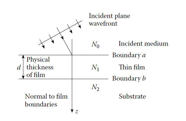
Plane wave incident on a thin film.
The interfaces between the film and the incident medium and the substrate, denoted by the symbols \(a\) and \(b\), can be treated in exactly the same way as the simple boundary already discussed. We consider the tangential components of the fields. There is no negative-going wave in the substrate, and the waves in the film can be summed into one resultant positive-going wave and one resultant negative-going wave. At this interface, then, the tangential components of \(E\) and \(H\) are:
\[
E_b = E_b^+ + E_b^-, \quad H_b = \frac{1}{\eta_1}(E_b^+ – E_b^-),
\]
where we are neglecting the common phase factors and where \(E_b\) and \(H_b\) represent the resultants. Hence:
\[
E_b^+ = \frac{1}{2} \left(E_b + \eta_1 H_b\right), \quad E_b^- = \frac{1}{2} \left(E_b – \eta_1 H_b\right),
\]
(Equations 2.92 and 2.93)
\[
H_b^+ = \frac{1}{2 \eta_1} \left(E_b + \eta_1 H_b\right), \quad H_b^- = \frac{1}{2 \eta_1} \left(E_b – \eta_1 H_b\right).
\]
(Equations 2.94 and 2.95)
The fields at the other interface (a), at the same instant and at a point with identical \(x\) and \(y\) coordinates, can be determined by altering the phase factors of the waves to allow for a shift in the \(z\)-coordinate from 0 to \(-d\). The phase factor of the positive-going wave will be multiplied by \(\exp(i\delta)\), where:
\[
\delta = \frac{2\pi N_1 d \cos\vartheta_1}{\lambda},
\]
and \(\vartheta_1\) may be complex, while the negative-going phase factor will be multiplied by \(\exp(-i\delta)\). We imply that this is a valid procedure when we say that the film is thin.
The values of \(E\) and \(H\) at the interface are now, using Equations 2.92 through 2.95:
\[
E_a^+ = E_b^+ e^{i\delta}, \quad E_a^- = E_b^- e^{-i\delta},
\]
\[
H_a^+ = H_b^+ e^{i\delta}, \quad H_a^- = H_b^- e^{-i\delta}.
\]
Thus:
\[
E_a = E_a^+ + E_a^- = E_b^+ e^{i\delta} + E_b^- e^{-i\delta},
\]
\[
H_a = \frac{1}{\eta_1}(E_b^+ e^{i\delta} – E_b^- e^{-i\delta}).
\]
These two simultaneous equations can be written in matrix notation as:
\[\begin{bmatrix}E_a \\H_a\end{bmatrix} \begin{bmatrix}
\cos\delta & i\sin\delta/\eta_1 \\ i\eta_1 \sin\delta & \cos\delta \end{bmatrix} \begin{bmatrix} E_b \\ H_b\end{bmatrix}\]
(Equation 2.96)
Because the tangential components of \(E\) and \(H\) are continuous across a boundary and because there is only a positive-going wave in the substrate, this relationship connects the tangential components of \(E\) and \(H\) at the incident interface with the tangential components of \(E\) and \(H\) transmitted through the final interface. The \(2 \times 2\) matrix on the right-hand side of Equation 2.96 is known as the characteristic matrix of the thin film.
We define the input optical admittance of the assembly by analogy with Equation 2.67 as:
\[
Y = \frac{H_a}{E_a},
\]
(Equation 2.97)
when the problem becomes merely that of finding the reflectance of a simple interface between an incident medium of admittance \(\eta_0\) and a medium of admittance \(Y\), i.e.,
\[
\rho = \frac{\eta_0 – Y}{\eta_0 + Y}, \quad R = \left|\frac{\eta_0 – Y}{\eta_0 + Y}\right|^2.
\]
(Equations 2.98)
We can normalize Equation 2.96 by dividing through by \(E_b\) to give:
\[\begin{bmatrix} E_a/E_b \\ H_a/E_b \end{bmatrix}\begin{bmatrix}
\cos\delta & i\sin\delta/\eta_1 \\ i\eta_1 \sin\delta & \cos\delta \end{bmatrix} \begin{bmatrix} 1 \\
H_b/E_b \end{bmatrix} \]
(Equation 2.99)
\(B\) and \(C\), the normalized electric and magnetic fields at the front interface, are the quantities from which we will extract the properties of the thin-film system. Clearly, from Equations 2.97 and 2.99, we can write:
\[
Y = \frac{H_a}{E_a} = \frac{\eta_1 \cos\delta + i\eta_1 \sin\delta}{\cos\delta + i(\sin\delta/\eta_1)}.
\]
(Equation 2.100)
From Equations 2.100 and 2.98, we can calculate the reflectance.
\[
\begin{bmatrix}
B \\
C
\end{bmatrix}
\]
is known as the characteristic matrix of the assembly.
4 The Reflectance of an Assembly of Thin Films
Let another film be added to the single film of the previous section so that the final interface is now denoted by \(c\), as shown in Figure 2.7. The characteristic matrix of the film nearest the substrate is:
\[\begin{bmatrix} \cos\delta_2 & i \sin\delta_2 / \eta_2 \\ i \eta_2 \sin\delta_2 & \cos\delta_2 \end{bmatrix}\]
(Equation 2.101)

Figure 2.7
Notation for two films on a surface.
From Equation 2.96:
\[ \begin{bmatrix} E_b \\ H_b \end{bmatrix} \begin{bmatrix} \cos\delta_2 & i \sin\delta_2 / \eta_2 \\ i \eta_2 \sin\delta_2 & \cos\delta_2 \end{bmatrix} \begin{bmatrix} E_c \\ H_c \end{bmatrix}\]
We can apply Equation 2.96 again to give the parameters at interface \(a\), i.e.,
\[\begin{bmatrix} E_a \\ H_a \end{bmatrix} \begin{bmatrix} \cos\delta_1 & i \sin\delta_1 / \eta_1 \\ i \eta_1 \sin\delta_1 & \cos\delta_1 \end{bmatrix} \begin{bmatrix} \cos\delta_2 & i \sin\delta_2 / \eta_2 \\ i \eta_2 \sin\delta_2 & \cos\delta_2 \end{bmatrix} \begin{bmatrix} E_c \\ H_c \end{bmatrix} \]
The characteristic matrix of the assembly, by analogy with Equation 2.99, is:
\[\begin{bmatrix} B \\ C \end{bmatrix} \begin{bmatrix} \cos\delta_1 & i \sin\delta_1 / \eta_1 \\ i \eta_1 \sin\delta_1 & \cos\delta_1 \end{bmatrix} \begin{bmatrix} \cos\delta_2 & i \sin\delta_2 / \eta_2 \\ i \eta_2 \sin\delta_2 & \cos\delta_2 \end{bmatrix} \]
The input admittance \(Y\) is, as before, \(C / B\), and the amplitude reflection coefficient and the reflectance are, from Equation 2.98:
\[
\rho = \frac{\eta_0 – Y}{\eta_0 + Y}, \quad R = \left|\frac{\eta_0 – Y}{\eta_0 + Y}\right|^2.
\]
(Equation 2.102)
This result can be immediately extended to the general case of an assembly of \(q\) layers, where the characteristic matrix is simply the product of the individual matrices taken in the correct order, i.e.,
\[ \begin{bmatrix} B \\ C \end{bmatrix} \prod_{r=1}^q \begin{bmatrix} \cos\delta_r & i \sin\delta_r / \eta_r \\
i \eta_r \sin\delta_r & \cos\delta_r \end{bmatrix} \]
(Equation 2.103)
Here:
\[
\delta_r = \frac{2\pi}{\lambda} d_r \sqrt{n_r^2 – k_r^2 – n_0^2 \sin^2\vartheta_0 – i 2 n_r k_r},
\]
(Equation 2.105)
with the correct solution in the fourth quadrant.
The admittance for \(s\)-polarization (TE) is:
\[
\eta_{rs} = Y \sqrt{n_r^2 – k_r^2 – n_0^2 \sin^2\vartheta_0 – i 2 n_r k_r},
\]
(Equation 2.106)
and for \(p\)-polarization (TM):
\[
\eta_{rp} = \frac{Y^2}{\eta_{rs}^2} = Y^2 (n_r – i k_r)^2.
\]
(Equation 2.107)
The determinant of the characteristic matrix for a thin film is unity, ensuring consistent phase relationships and avoiding difficulties with signs and quadrants.
The phase shift associated with the reflected beam can be examined by expressing \(Y = a + ib\), where \(a\) and \(b\) are real and \(\eta_0\) is real. The reflection coefficient becomes:
\[
\rho = \frac{\eta_0 – (a + ib)}{\eta_0 + (a + ib)} = \frac{(\eta_0 – a) – i b}{(\eta_0 + a) + i b},
\]
so the phase shift \(\phi\) is given by:
\[
\tan\phi = \frac{-2b\eta_0}{(\eta_0^2 – a^2 – b^2)}.
\]
(Equation 2.108)
This must be interpreted based on the sign conventions established in Figure 2.3. The numerator and denominator should be preserved as shown to ensure the quadrant is uniquely specified. The rule is simple: the quadrant is determined by the vector associated with \(\rho\), with the denominator as the \(x\)-coordinate and the numerator as the \(y\)-coordinate. Note that the reference surface for phase shift calculation is the front surface of the multilayer.

5 Reflectance, Transmittance, and Absorptance
Sufficient information is included in Equation 2.103 to allow the transmittance and absorptance of a thin-film assembly to be calculated. For this to have a physical meaning, as we have already seen, the incident medium should be transparent, that is, \(\eta_0\) must be real. The substrate need not be transparent, but the transmittance calculated will be the transmittance into, rather than through, the substrate.
First, we calculate the net irradiance at the exit side of the assembly, which we take as the (k)th interface. This is given by:
\[
I_k = \frac{1}{2} \text{Re}(E_k H_k^*),
\]
where, again, we are dealing with the component of irradiance normal to the interfaces. Using the relationship between electric and magnetic fields:
\[
I_k = \frac{1}{2} \text{Re} \left( \frac{|E_k|^2}{\eta_k} \right),
\]
(Equation 2.109)
where \(\eta_k\) is the admittance of the medium at the exit side.
If the characteristic matrix of the assembly is:
\[
\begin{bmatrix}
B \\
C
\end{bmatrix},
\]
then the net irradiance at the entrance to the assembly is:
\[
I_a = \frac{1}{2} \text{Re}(BC^*).
\]
*(Equation 2.110)*
Let the incident irradiance be denoted by \(I_i\). Then Equation 2.110 represents the irradiance actually entering the assembly, which is \((1 – R)I_i\):
\[
(1 – R)I_i = \frac{1}{2} \text{Re}(BC^*),
\]
so:
\[
I_i = \frac{\text{Re}(BC^*)}{2(1 – R)}.
\]
Equation 2.109 represents the irradiance leaving the assembly and entering the substrate, and so the transmittance \(T\) is:
\[
T = \frac{I_k}{I_i} = \frac{\text{Re}(\eta_m)}{\text{Re}(BC^*)} (1 – R).
\]
*(Equation 2.111)*
The absorptance \(A\) in the multilayer is connected with \(R\) and \(T\) by the relationship:
\[
1 = R + T + A,
\]
so that:
\[
A = 1 – R – T = 1 – R – \frac{\text{Re}(\eta_m)}{\text{Re}(BC^*)} (1 – R).
\]
*(Equation 2.112)*
In the absence of absorption in any of the layers, it can readily be shown that the above expressions are consistent with \(A = 0\) and \(T + R = 1\), since the individual film matrices have determinants of unity, and the product of any number of these matrices will also have a determinant of unity. The product of the matrices can be expressed as:
\[
\begin{bmatrix}
\alpha & \beta \\
\gamma & \delta
\end{bmatrix},
\]
where \(\alpha\delta + \gamma\beta = 1\) and, because there is no absorption, \(\alpha\), \(\beta\), \(\gamma\), and \(\delta\) are all real.
From Equation 2.98:
\[
R = \left|\frac{\eta_0 – Y}{\eta_0 + Y}\right|^2 = \frac{(\eta_0 – Y)(\eta_0 – Y^)}{(\eta_0 + Y)(\eta_0 + Y^)}.
\]
(Equation 2.113)
Expanding the terms, we find:
\[
1 – R = \frac{2 \eta_0 \text{Re}(Y)}{|\eta_0 + Y|^2}.
\]
(Equation 2.114)
Inserting this result into Equation 2.111, we obtain:
\[
T = \frac{4\eta_0 \text{Re}(\eta_m)}{|\eta_0 + Y|^2}.
\]
(Equation 2.115)
And in Equation 2.112:
\[
A = 1 – \frac{4\eta_0 \text{Re}(\eta_m)}{|\eta_0 + Y|^2} – R.
\]
(Equation 2.116)
Equations 2.113, 2.115, and 2.116 are the most useful forms of the expressions for \(R\), \(T\), and \(A\).
An important quantity that we shall discuss in a later section of this chapter is \(T/(1 – R)\), known as the potential transmittance \(\psi\). From Equation 2.111:
\[
\psi = \frac{T}{1 – R} = \frac{\text{Re}(\eta_m)}{\text{Re}(BC^*)}.
\]
*(Equation 2.117)*
The phase change on reflection (Equation 2.108) can also be expressed in a compatible form:
\[
\phi = \arctan\left(\frac{\text{Im}(\eta_m BC^* – \eta_m^* CB^)}{2 \text{Re}(\eta_m BC^)}\right).
\]
(Equation 2.118)
The quadrant of \(\phi\) is determined by the same arrangement of signs for the numerator and denominator as in Equation 2.108. The phase change on reflection is measured at the front surface of the multilayer.
The phase shift on transmission is sometimes important. Denoting the phase shift by \(\zeta\), it is defined as the difference in phase between the resultant transmitted wave (as it enters the emergent medium) and the incident wave at the front surface (as it enters the multilayer). Using normalized amplitudes for the electric field:
\[
E_i + E_r = \frac{B}{C} (\eta_0 – \eta_0).
\]
Eliminating \(E_r\), we find:
\[
E_i = \frac{1}{2}\left(\frac{B}{C}\right) + \eta_0.
\]
Thus, the amplitude transmission coefficient becomes:
\[
\tau = \frac{2\eta_0}{\eta_0 + \frac{B}{C}}.
\]
The phase shift is then given by:
\[
\zeta = \arctan\left(\frac{\text{Im}(B/C)}{\text{Re}(B/C)}\right).
\]
(Equation 2.119)
As before, it is essential to preserve the signs of the numerator and denominator to determine the quadrant correctly.
6 Units
We have been using the SI units in the work so far. In this system, \(y\), \(\eta\), and \(Y\) are measured in siemens. Much of the thin-film literature, especially the earlier works, has been written in Gaussian units.
In Gaussian units, \(Y\), the admittance of free space, is unity. Thus, since \(y = NY\), \(y\) (the optical admittance) and \(N\) (the refractive index) are numerically equal at normal incidence, although \(N\) is a dimensionless quantity. The position is different in SI units, where \(Y\) is:
\[
Y = 2.6544 \times 10^{-3} \text{ S}.
\]
We could, if we choose, measure \(y\) and \(\eta\) in units of \(Y\) (in siemens), which we can call free space units. In this case, \(y\) becomes numerically equal to \(N\), just as in the Gaussian system. This is a perfectly valid procedure, and all the expressions for ratioed quantities—such as reflectance, transmittance, absorptance, and potential transmittance—remain unchanged. This applies particularly to Equations 2.103 and 2.113 through 2.117.
When calculating absolute rather than relative irradiance, or when deriving the magnetic field, care must be taken to ensure consistent units. Specifically, Equation 2.96 becomes:
\[\begin{bmatrix} E_a / Y \\ H_a / Y \end{bmatrix} = \begin{bmatrix} \cos\delta_1 & i \sin\delta_1 / \eta_1 \\
i \eta_1 \sin\delta_1 & \cos\delta_1 \end{bmatrix} \begin{bmatrix} E_b / Y \\ H_b / Y \end{bmatrix} \]
(Equation 2.120)
where \(\eta\) is now measured in free space units.
In most cases in this book, either arrangement can be used. In some cases, particularly where we use graphical techniques, we shall use free space units, because otherwise the scales become quite cumbersome.
7 Summary of Important Results
We have now covered all the basic theory necessary for understanding the remainder of the book. It has been a somewhat long and involved discussion, so we now summarize the principal results. The statement numbers refer to those in the text where the particular quantities were originally introduced.
- Refractive Index:
- Defined as the ratio of the velocity of light in free space \((c)\) to the velocity of light in the medium \((v)\):
\[
N = \frac{c}{v} = n – ik,
\]
(Equation 2.19)
where \(n\) is the real refractive index, and \(k\) is the extinction coefficient. \(N\) is a function of wavelength \(\lambda\). - \(k\) is related to the absorption coefficient \(\alpha\):
\[
\alpha = \frac{4\pi k}{\lambda}.
\]
(Equation 2.35) - Electromagnetic Waves:
- A homogeneous, plane, linearly polarized harmonic wave is represented as:
\[
E = E \exp\left[i\omega t – \frac{2\pi N}{\lambda}z + \phi\right],
\]
(Equation 2.22)
and similarly for the magnetic field:
\[
H = H \exp\left[i\omega t – \frac{2\pi N}{\lambda}z + \phi’\right].
\]
(Equation 2.121) - The phase change after traversing a distance \(d\) of the medium is:
\[
-\frac{2\pi}{\lambda}Nd = -\frac{2\pi}{\lambda}nd – i\frac{2\pi}{\lambda}kd,
\]
(Equation 2.122)
where the imaginary part corresponds to amplitude reduction. - Optical Admittance:
- Defined as:
\[
y = \frac{H}{E},
\]
which is usually complex. In free space:
\[
Y = 2.6544 \times 10^{-3} \text{ S}.
\]
(Equation 2.123) - For a medium:
\[
y = NY.
\]
(Equation 2.124) - Irradiance:
- Defined as the mean energy flow per unit area:
\[
I = \frac{1}{2} \text{Re}(E H^*).
\]
*(Equation 2.33)*
Or:
\[
I = \frac{1}{2} \frac{n |E|^2}{Y}.
\]
(Equation 2.125) - At a Boundary:
- For normal incidence:
- Amplitude reflection coefficient:
\[
\rho = \frac{y_0 – y_1}{y_0 + y_1}.
\]
(Equation 2.73) - Amplitude transmission coefficient:
\[
\tau = \frac{2y_0}{y_0 + y_1}.
\]
(Equation 2.74) - Reflectance:
\[
R = |\rho|^2 = \frac{(y_0 – y_1)(y_0 – y_1)^*}{(y_0 + y_1)(y_0 + y_1)^*}.
\]
(Equation 2.77) - Transmittance:
\[
T = \frac{4y_0 \text{Re}(y_1)}{(y_0 + y_1)(y_0 + y_1)^*}.
\]
*(Equation 2.78)*
- Amplitude reflection coefficient:
- Oblique Incidence:
- For \(p\)-polarized (TM) and \(s\)-polarized (TE) waves:
\[
\eta_p = \frac{N}{\cos\vartheta}, \quad \eta_s = N \cos\vartheta,
\]
where \(\vartheta\) is the angle of incidence or refraction.
(Equation 2.126)- Reflection and transmission coefficients:
\[
\rho = \frac{\eta_0 – \eta_1}{\eta_0 + \eta_1}, \quad \tau = \frac{2\eta_0}{\eta_0 + \eta_1}.
\]
(Equations 2.88, 2.89) - Reflectance and transmittance:
\[
R = \left|\frac{\eta_0 – \eta_1}{\eta_0 + \eta_1}\right|^2, \quad T = \frac{4\eta_0 \text{Re}(\eta_1)}{|\eta_0 + \eta_1|^2}.
\]
(Equations 2.90, 2.91)
- Reflection and transmission coefficients:
- Assembly of Thin Films:
- Admittance of the multilayer:
\[
Y = \frac{C}{B},
\]
(Equation 2.127)
where \(B\) and \(C\) are derived from the characteristic matrix. - Reflectance, transmittance, and absorptance:
\[
R = \frac{(B – \eta_0 C)(B – \eta_0 C)^*}{(B + \eta_0 C)(B + \eta_0 C)^*},
\]
(Equation 2.113) \[
T = \frac{4\eta_0 \text{Re}(\eta_m)}{(B + \eta_0 C)(B + \eta_0 C)^*},
\]
*(Equation 2.115)* \[
A = 1 – R – T.
\]
(Equation 2.116) - Phase Shifts:
- Reflection:
\[
\phi = \arctan\left(\frac{\text{Im}(\eta_m BC^* – \eta_m^* CB^)}{\text{Re}(\eta_m BC^ – \eta_m^* CB^*)}\right).
\]
*(Equation 2.118)* - Transmission:
\[
\zeta = \arctan\left(\frac{\text{Im}(B/C)}{\text{Re}(B/C)}\right).
\]
(Equation 2.119)
For numerical calculations, automated tools are often necessary due to the complexity of multilayer structures. Approximate and graphical methods can offer insights into their behavior and design limitations.

8 Potential Transmittance
Transmittance is a less accessible parameter from the theoretical perspective than reflectance. Reflectance is directly a function of the admittance of the front surface of the multilayer, whereas calculating transmittance requires additional information. A useful related concept is potential transmittance, which is more accessible theoretically.
The potential transmittance of a layer or an assembly of layers is the ratio of the irradiance leaving by the rear (exit) interface to that entering by the front interface. This concept was introduced by Berning and Turner and is especially useful in designing metal-dielectric filters and calculating losses in all-dielectric multilayers. Potential transmittance is denoted by \(\psi\) and is given by:
\[
\psi = \frac{I_{\text{exit}}}{I_{\text{enter}}} = \frac{T}{1 – R},
\]
(Equation 2.129)
where \(T\) is the transmittance and \(R\) is the reflectance. This represents the ratio between the irradiance leaving the assembly and the net irradiance actually entering, defined as the difference between the incident and reflected irradiances.
The potential transmittance of a series of subassemblies of layers is simply the product of the individual potential transmittances. Figure 2.8 illustrates a series of film subunits making up a complete system. Clearly:
\[
\psi = \psi_1 \cdot \psi_2 \cdot \psi_3 = \frac{I_e}{I_a} = \frac{I_d}{I_b} \cdot \frac{I_c}{I_a},
\]
(Equation 2.130)
where the irradiances correspond to the respective interfaces.

Figure 2.8
(a) An assembly of thin films. (b) The potential transmittance of an assembly of thin film
..consisting of a number of subunits.
Properties of Potential Transmittance
- The potential transmittance depends on the parameters of the layer or combination of layers involved, and on the characteristics of the structure at the exit interface.
- It represents the maximum transmittance achievable if there were no reflection losses, serving as an ideal measure of transmittance.
- By definition, the potential transmittance is unaffected by any transparent structure deposited over the front surface, though it is affected by changes at the exit interface.
To ensure the transmittance equals the potential transmittance, layers added to the front surface must maximize the irradiance entering the assembly. This implies reducing reflectance to zero, e.g., by adding an antireflection coating.
Matrix Representation of Potential Transmittance
Reflectance is defined only in media without absorption, and irradiances must be interpreted as the net irradiance passing through the respective interface. Using the characteristic matrix notation, where \(B\) and \(C\) denote the normalized electric and magnetic fields at any interface, the net normalized irradiance is:
\[
\text{Irradiance} \propto \text{Re}(BC^*).
\]
Thus, in terms of \(B\) and \(C\), potential transmittance becomes:
\[
\psi = \frac{\text{Re}(BC^{\text{exit}})}{\text{Re}(BC^{\text{enter}})}.
\]
(Equation 2.132)
Consider a multilayer assembly with matrices for subassemblies \(M_a\), \(M_b\), and \(M_c\), and matrices for other layers denoted by \(M_p\), \(M_q\), etc.:
\[ \begin{bmatrix} B_i \\ C_i \end{bmatrix}=[M_a] [M_b] [M_c] \cdots \begin{bmatrix} B_e \\ C_e
\end{bmatrix} \]
(Equation 2.131)
where \([M_a][M_b][M_c]\) is the subassembly of interest, and \([M_p][M_q]\) represents the remaining structure.
Simplified Expression
By dividing through by \(B_e\):
\[ \begin{bmatrix} B_i’ \\ C_i’ \end{bmatrix} = [M_a] [M_b] [M_c] \begin{bmatrix} 1 \\ Y_e
\end{bmatrix} \]
where:
\[
Y_e = \frac{C_e}{B_e}, \quad B_i’ = \frac{B_i}{B_e}, \quad C_i’ = \frac{C_i}{C_e}.
\]
The potential transmittance is then:
\[
\psi = \frac{\text{Re}(B_e C_e^*)}{\text{Re}(B_i C_i^*)}
\]
which is consistent with Equation 2.132. Thus, the potential transmittance of any subassembly is determined solely by the characteristics of the subassembly and the optical admittance at the exit interface.
9 A Theorem on the Transmittance of a Thin-Film Assembly
The transmittance of a thin-film assembly is independent of the direction of propagation of the light. This applies regardless of whether the layers are absorbing.
A proof of this result, from Abelès, who developed the matrix approach to thin-film analysis, follows quickly from the properties of the matrices.
Proof
Let the matrices of the various layers in the assembly be denoted by:
\[
M_1, M_2, \dots, M_q,
\]
and let the two massive media on either side of the assembly be transparent. The two matrix products corresponding to the two possible directions of propagation can be written as:
\[
M = [M_1][M_2][M_3]\dots[M_q],
\]
and for reverse propagation:
\[
M’ = [M_q][M_{q-1}]\dots[M_2][M_1].
\]
Because the form of the matrices is such that the diagonal terms are equal, regardless of whether there is absorption, we can show that if we write:
\[M = \begin{bmatrix} a_{11} & a_{12} \\ a_{21} & a_{22} \end{bmatrix}, \quad M’ = \begin{bmatrix}
a'{11} & a'{12} \\ a'{21} & a'{22} \end{bmatrix}\]
then:
\[
a_{ij} = a'{ij} \quad (i \neq j), \quad a{11} = a'{22}, \quad a{22} = a’_{11}.
\]
This property can be proved by induction.
Characteristic Matrix in Both Directions
Let the medium on one side of the assembly be \(\eta_0\) and on the other side \(\eta_m\), where \(\eta_0\) is adjacent to layer 1.
- First Direction:
Using the characteristic matrix for the first direction:
\[
\begin{bmatrix}
B \\
C \end{bmatrix} M
\begin{bmatrix}
1 \\
\eta_m
\end{bmatrix},
\]
we have:
\[
B = a_{11} + a_{12}\eta_m, \quad C = a_{21} + a_{22}\eta_m.
\] - Second Direction:
For reverse propagation:
\[
\begin{bmatrix}
B \\
C
\end{bmatrix}
=
M’
\begin{bmatrix}
1 \\
\eta_0
\end{bmatrix},
\]
we have:
\[
B = a'{11} + a'{12}\eta_0, \quad C = a'{21} + a'{22}\eta_0.
\]
By the symmetry properties of the matrices:
\[
B = a_{22} + a_{12}\eta_0, \quad C = a_{21} + a_{11}\eta_0.
\]
Transmittance
Using Equation 2.115, the transmittance for the first direction is:
\[
T = \frac{4\eta_0 \text{Re}(\eta_m)}{|a_{11} + a_{12}\eta_m|^2 + |a_{21} + a_{22}\eta_m|^2}.
\]
For the second direction:
\[
T = \frac{4\eta_m \text{Re}(\eta_0)}{|a_{22} + a_{12}\eta_0|^2 + |a_{21} + a_{11}\eta_0|^2}.
\]
These two expressions are identical, proving that the transmittance is independent of the direction of propagation.
Implications
- Reflectance: The reflectance of an assembly depends on the direction of propagation only if there is absorption in the layers. If the layers are non-absorbing, the reflectance is the same in both directions.
- One-Way Mirrors: This theorem implies that a true one-way mirror, which allows light to pass in one direction only, cannot be constructed from simple optical thin films. Practical one-way mirrors rely on differences in illumination conditions on either side rather than inherent optical properties.
10 Coherence
Coherence quantifies the ability of a system to produce detectable interference effects. While it is often used to describe the properties of a beam of light, it is more appropriately considered a property of the complete optical system.
The term coherent describes the presence of maximum interference effects, incoherent refers to their complete absence, and cases in between are described as partially coherent. Here, we briefly examine aspects of coherence that are significant in optical coating applications.
Stationary Phenomena
In our discussion, we assume stationary phenomena. This means that while waves may exhibit variations, their statistical properties remain constant over time. Such phenomena can be averaged over a sufficiently long time or across many cases, as though conducting an experiment.
Since interactions are linear, we represent an arbitrary wave as a spectrum of harmonic waves. Consider two beams derived from a single spectral element:
- Two linearly polarized plane waves with identical polarization propagating along the \(z\)-direction have complex amplitudes \(E_1\) and \(E_2\).
- Let their phases at \(z = 0\) and \(t = 0\) be \(\phi_1\) and \(\phi_2\), contained in their complex amplitudes.
The resultant irradiance, when the waves combine, is:
\[
I = y \big| E_1 + E_2 \big|^2 = y \Big( |E_1|^2 + |E_2|^2 + 2 \text{Re}(E_1E_2^*) \Big).
\]
*(Equation 2.133)*
This can also be expressed as:
\[
I = I_1 + I_2 + 2\sqrt{I_1 I_2} \cos(\phi_2 – \phi_1),
\]
(Equation 2.134)
where \(I_1 = y |E_1|^2\), \(I_2 = y |E_2|^2\), and the interference term depends on the phase difference.
Coherence in Complex Systems
In a real system with multiple light waves of varying frequencies, phases, and amplitudes, the resultant irradiance becomes a sum of individual irradiances plus interference terms. Depending on the spread of parameters, the interference term can:
- Remain strong: Coherent.
- Cancel out completely: Incoherent.
- Partially cancel: Partially coherent.
Factors such as variations in the light source or system properties (e.g., film thickness variations) can affect coherence. Substrates are typically thick and variable enough to exhibit incoherent behavior, while thin films can maintain coherence.
Coherence Parameters
To quantify coherence, we consider:
- Coherence Length: The distance along the light’s propagation direction where interference fringes just disappear.
- Coherence Area: The area over which the fringes disappear when light is taken from different parts of a beam.
- Coherence Time: The time delay at which interference fringes disappear. It is related to coherence length as:
\[
\text{Coherence Time} = \frac{\text{Coherence Length}}{c},
\]
where \(c = 299,792.458 \, \text{nm/fs}\).
Spectral Coherence
For light expressed as a continuous spectrum centered at \(\lambda\) with a bandwidth \(\Delta\lambda\), the coherence length can be approximated as:
\[
\text{Coherence Length} = \frac{\lambda^2}{\Delta\lambda}.
\]
(Equation 2.136)
The corresponding coherence time is:
\[
\text{Coherence Time} = \frac{\lambda^2}{c \Delta\lambda}.
\]
(Equation 2.137)
For cones of illumination with semiangle \(\vartheta\), an approximate two-dimensional model gives:
\[
\text{Coherence Length} = \frac{\lambda}{2(1 – \cos\vartheta)} \approx \frac{\lambda}{\vartheta^2},
\]
(Equation 2.139)
or in degrees:
\[
\text{Coherence Length} \approx \frac{7 \times 10^3 \, \lambda}{\vartheta^2}.
\]
(Equation 2.140)
For a medium with refractive index \(n_1\) and incident medium \(n_0\), we correct for the cone angle as:
\[
\text{Coherence Length} = \frac{7 \times 10^3 \, \lambda}{n_1^2 \vartheta^2}.
\]
(Equation 2.141)
When multiple effects (e.g., cone and bandwidth) influence coherence, the combined coherence length is:
\[
\frac{1}{L^2} = \frac{1}{L_a^2} + \frac{1}{L_b^2} + \dots
\]
(Equation 2.142)
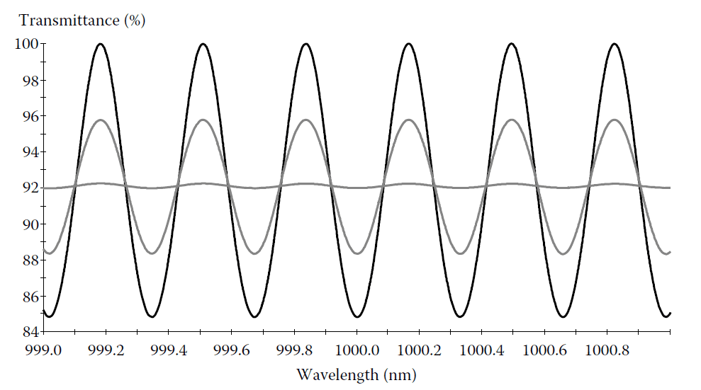
The appearance of fringes in a perfectly parallel 1-mm-thick glass substrate illuminated with light
of zero bandwidth, 0.2-nm bandwidth (coherence length 5 mm), and 2-nm bandwidth (0.5 mm
coherence length). The fringes show reducing amplitude with decreasing coherence length.
Fringe Visibility
For general waves, the mutual coherence function is defined as:
\[
\Gamma_{12}(\tau) = \lim_{T \to \infty} \frac{1}{T} \int_{-T/2}^{T/2} E_1(t)E_2^*(t+\tau) \, dt.
\]
*(Equation 2.143)*
The complex degree of coherence is:
\[
\gamma_{12}(\tau) = \frac{\Gamma_{12}(\tau)}{\sqrt{\Gamma_{11}(0)\Gamma_{22}(0)}}.
\]
(Equation 2.144)
The irradiance becomes:
\[
I = I_1 + I_2 + 2 \sqrt{I_1 I_2} \, \text{Re}(\gamma_{12}(\tau)).
\]
(Equation 2.145)
Fringe visibility is defined as:
\[
V = \frac{I_{\max} – I_{\min}}{I_{\max} + I_{\min}} = |\gamma_{12}(\tau)|.
\]
(Equation 2.147)
Practical Considerations
While coherence time and length are practical for explaining phenomena, the real system is never perfectly coherent. In this book, we assume:
- Complete coherence for thin-film coatings.
- Complete incoherence for substrates.
This treatment balances theoretical rigor with practical relevance for optical coating applications.
11 Incoherent Reflection at Two or More Surfaces
So far, we have treated substrates as one-sided slabs of infinite depth. In practical cases, substrates usually have finite depth, with rear surfaces that reflect some energy and affect the performance of the assembly.
Conditions for Incoherence
- Substrate depth is typically much greater than the wavelength of light.
- Variations in surface flatness and parallelism are appreciable fractions of a wavelength.
- Incident light is often not well collimated.
Under these conditions, interference effects between light reflected at the front and rear surfaces of the substrate are not observable with a finite aperture. This makes the substrate thick, and the coherence length is small compared to the double traversal of the substrate. As a result, we describe the addition of waves as incoherent, meaning the interference term vanishes, leaving a sum of irradiances rather than a vector sum of amplitudes.
Irradiance Sum
The symbols are illustrated in Figure 2.10, where waves are reflected successively at the front and rear surfaces. The sum of the irradiances is given by:
\[
R_a = R_a + R_b T_a T_a + R_a R_b^2 T_a^2 + \dots
\]
This simplifies to:
\[
R_a = R_a + \frac{R_b T_a^2}{1 – R_a R_b},
\]
where \(T_+\) and \(T_-\) are always identical. Thus:
\[
T_a^+ = T_a^- = T_a.
\]
The total reflectance becomes:
\[
R = R_a + \frac{T_a^2 R_b}{1 – R_a R_b}.
\]
If there is no absorption:
\[
R = R_a + R_b – R_a R_b.
\]
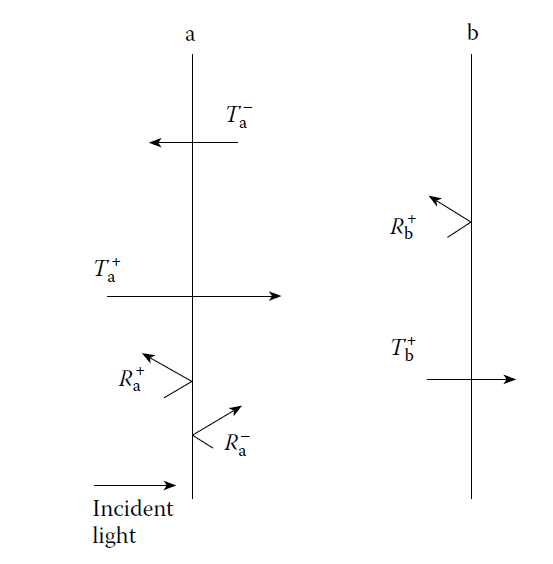
Symbols used in calculation of incoherent reflection at two or more surfaces.
Total Transmittance
The total transmittance is similarly given by:
\[
T = T_a T_b + T_a T_b R_a R_b + \dots,
\]
which simplifies to:
\[
T = T_a T_b (1 – R_a R_b).
\]
(Equation 2.148)
If there is no absorption, this further simplifies to:
\[
T = 1 – R.
\]
(Equation 2.149)
A nomogram can be constructed for solving Equation 2.149, as shown in Figure 2.11. The method uses intersecting axes for transmittance scales.
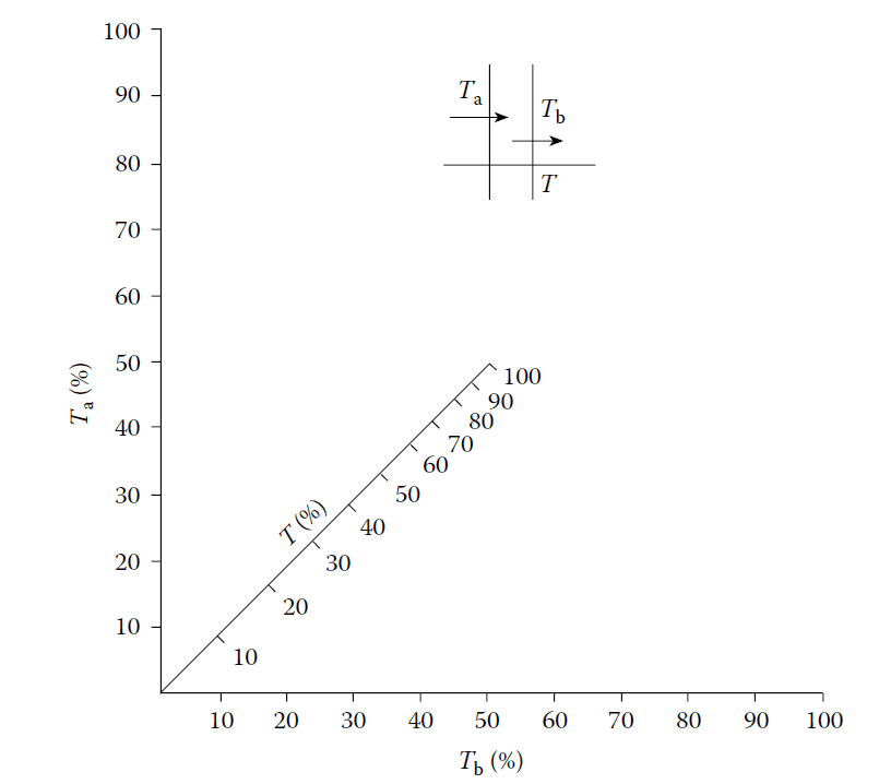
A nomogram for calculating the overall transmittance of a thick transparent plate given the
transmittance of each individual surface.
Multiple Substrates
For two substrates \((T_a, T_b, T_c, T_d)\):
- For the first substrate:
\[
\frac{1}{T_1} = \frac{1}{T_a} + \frac{1}{T_b} – 1.
\] - For the second substrate:
\[
\frac{1}{T_2} = \frac{1}{T_c} + \frac{1}{T_d} – 1.
\]
The total transmittance through all four surfaces is:
\[
\frac{1}{T} = \frac{1}{T_1} + \frac{1}{T_2} – 1,
\]
or:
\[
T = \frac{1}{\frac{1}{T_a} + \frac{1}{T_b} + \frac{1}{T_c} + \frac{1}{T_d} – 3}.
\]
(Equation 2.150)
Matrix Formulation
For a more efficient method, Baumeister et al. proposed a matrix formulation based on irradiance flows. This approach assumes negligible absorption between the coated surfaces. The symbols are illustrated in Figure 2.12.
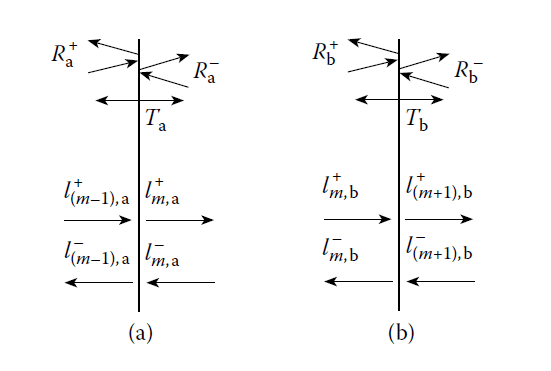
Symbols defining two successive coatings (a) and (b) with intervening medium in a stack.
Matrix Relations
- Across coating (b), the relations are: \[
I_m^+ = T_b I_m^+ + R_b I_m^-, \quad I_m^- = R_b I_m^+ + T_b I_m^-.
\] In matrix form: \[
\begin{bmatrix}
I_m^- \\
I_m^+ \end{bmatrix} = \begin{bmatrix}
R_b & T_b \\
T_b & R_b
\end{bmatrix}
\begin{bmatrix}
I_m^+ \\
I_m^-
\end{bmatrix}.
\]
(Equation 2.151) - Through medium \(m\) with transmittance \(T_\text{mint}\), the relation becomes: \[
\begin{bmatrix}
I_m^- \\
I_m^+ \end{bmatrix} = \begin{bmatrix}
T_\text{mint} & 0 \\
0 & T_\text{mint}
\end{bmatrix}
\begin{bmatrix}
I_b^- \\
I_b^+
\end{bmatrix}.
\]
(Equation 2.152)
Iterative Calculation
By applying Equations 2.151 and 2.152 iteratively to all coatings and media in the system, the total transmittance and reflectance can be computed efficiently.