The Fabry–Perot Interferometer
First described in 1899 by Fabry and Perot, the interferometer bearing their names has profoundly influenced thin-film optics. It belongs to the class of multiple-beam interferometers, involving a large number of beams in the interference. The theory for these interferometers is similar, differing mainly in physical form. Their fringes are sharper than those in two-beam interferometers, improving both measuring accuracy and resolution. Multiple-beam interferometers are described in textbooks such as Born and Wolf.
Basic Structure and Theory
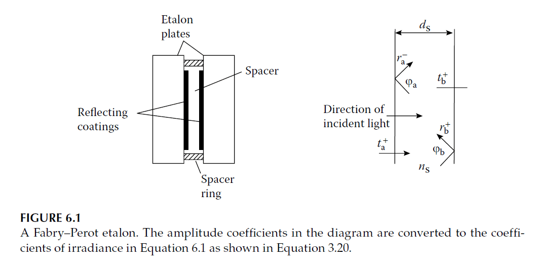
The heart of the Fabry–Perot interferometer is the etalon, consisting of two flat plates separated by a distance \( d_s \), aligned parallel to a very high degree of accuracy. The separation is typically maintained by a spacer ring made of Invar or quartz. The inner surfaces of the plates are coated to enhance reflectance.
Figure 6.1 shows a diagram of an etalon. The amplitude reflection and transmission coefficients are defined. The the transmission for a plane wave is:
\[
T = \frac{T_a T_b}{R_a R_b – 2 \sqrt{R_a R_b} \cos \delta + 1}
\]
where:
\[
\delta = \frac{2\pi n_s d_s \cos \theta_s}{\lambda}
\]
with \( d_s \) and \( n_s \) being the thickness and refractive index of the spacer layer, respectively. For simplicity, let \( R_a = R_b = R_s \) and \( \phi_a = \phi_b = 0 \). Then:
\[
T = \frac{T_s^2}{(1 – R_s)^2 + 4R_s \sin^2 \delta}
\]
Define the coefficient \( F \) as:
\[
F = \frac{4R_s}{(1 – R_s)^2}
\]
The equation for transmission becomes:
\[
T = \frac{1}{1 + F \sin^2 \delta}
\]
Characteristics of Transmission
If there is no absorption in the reflecting layers:
\[
1 – R_s = T_s
\]
\[
T = \frac{1}{1 + F \sin^2 \delta}
\]
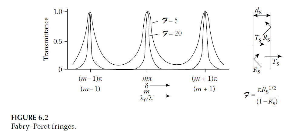
The transmission \( T \) is a maximum when \( \delta = m\pi \), where \( m = 0, \pm1, \pm2, \ldots \). The successive peaks are multiple-beam fringes, and \( m \) is the fringe order. Figure 6.2 shows \( T \) plotted against \( \delta \).
The finesse of the interferometer is defined as the ratio of the separation of adjacent fringes to their half-width. From Equation 6.5:
\[
\delta = \frac{1}{\sqrt{F}}
\]
The separation between successive fringes is \( \pi \), so:
\[
F = \frac{\pi \sqrt{F}}{\pi} = \frac{\pi R_s^{1/2}}{1 – R_s}
\]
Applications and Limitations
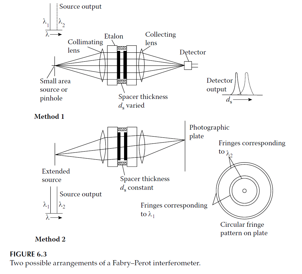
The Fabry–Perot interferometer is used to examine the fine structure of spectral lines. Fringes are produced by passing light through the interferometer. Figure 6.3 shows possible arrangements for either collimated light or varying the incidence angle \( \theta_s \).
Practical considerations limit finesse to around 25 or 50 due to plate imperfections. Flatness better than \( \lambda/100 \) at 546 nm is extremely challenging. Variations cause shifts in \( d_s \) and hence \( \delta \), reducing luminosity.
For a plate with a total thickness variation of \( \lambda/p \), the finesse is limited to \( p/2 \).
Resolving Power
The resolving power \( \lambda / \Delta \lambda \) is:
\[
\lambda / \Delta \lambda = mF
\]
where \( m \) is the fringe order. A low finesse can still achieve high resolution in high orders, but neighboring wavelengths overlap unless filtered. Thin-film filters or low-resolution etalons are often used for this purpose.
Absorption Effects
Including absorption in the coatings modifies Equation 6.4. Let \( A_s \) be the absorptance of each coating:
\[
1 = R_s + T_s + A_s
\]
Then:
\[
T = \frac{T_s^2}{(T_s + A_s)^2 + 4R_s \sin^2 \delta}
\]
Figure 6.4 shows curves of transmittance versus finesse, given coating absorptance. Silver performs best for visible and near-infrared ranges but declines at finesse values above 20. All-dielectric multilayer coatings significantly improve performance.
