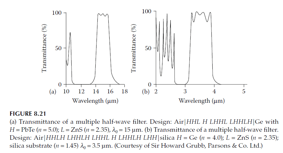
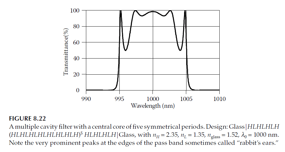
Figure 8.21b illustrates the square-shaped pass band of a multiple-cavity filter while highlighting a common problem: the “rabbit’s ears,” or prominent peaks at either side of the pass band. This issue worsens with an increasing number of periods, as shown in Figure 8.22.
Dispersion and Matching Challenges
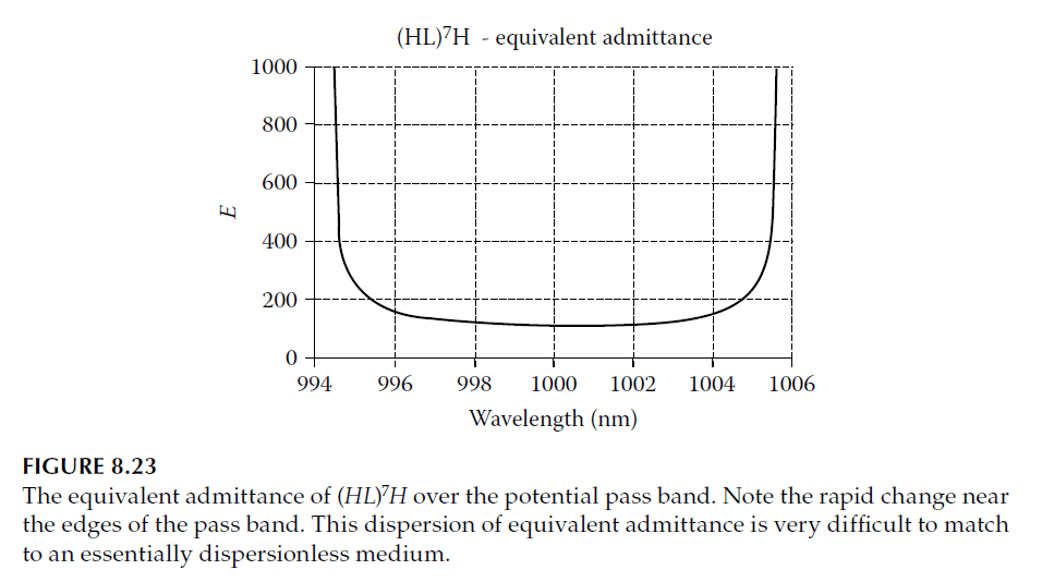
The peaks arise due to the dispersion of the equivalent admittance of the symmetrical period. Although design methods assume constant admittance across the pass band, the actual admittance varies significantly, approaching zero or infinity at the band edges (Figure 8.23). This challenge is analogous to edge filters, where ripple suppression near the edge requires matching systems with similar dispersion properties.
In band-pass filters, ripple suppression is required at both edges, making the design more complex. Inspired by shifted-period techniques, a potential solution involves creating a matching system with symmetrical dispersion to maintain effective matching even as equivalent admittance varies. Since symmetrical periods have an odd number of quarter-waves, their equivalent phase thickness at \(g = 1\) is an odd multiple of \(\pi/2\). This makes them viable as matching assemblies.
To implement this, we identify pairs of symmetrical periods with compatible admittance properties, allowing straightforward quarter-wave-based matching at the center of the pass band.
Using Higher-Order Periods
Adding half-wave layers to a symmetrical period does not alter its equivalent admittance at the pass-band center or the curvature of its admittance variation. Figure 8.24 shows examples such as:
– HLHLHLHLHLH
– HHHLHLHLHLHLHHH
– HLLLHLHLHLHLLLH
– HHHLLLHLHLHLHLLLHHH
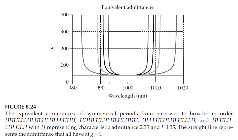
All these designs have the same admittance value (\(n_H^6 / n_L^5\)) at \(g = 1\), and broader curves remain closer to an odd number of quarter-waves as \(g\) varies. This property allows broader curves to match narrower ones to a notional medium with constant admittance (\(n_H^6 / n_L^5\)). The best-matching broader period is selected, and traditional quarter-wave matching to the external media completes the design.
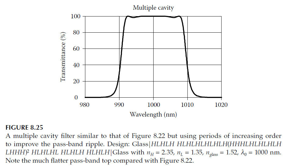
An example of this approach uses two periods, **HLHLHLHLHLH** and **HHHLHLHLHLHLHHH**, in the following configuration:
\[
\text{Glass | HLHLH HLHLHLHLHLH (HHHLHLHLHLHLHHH)}_q \text{ HLHLHLHLHLH HLHLH | Glass}
\]
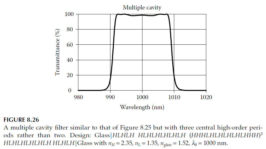
Performance characteristics for such filters are shown in Figures 8.25 and 8.26.
Bandwidth Calculation
The filter bandwidth is primarily determined by the highest-order periods. For a period expressed as:
\[
mABABA…BmA
\]
with \(2x + 1\) layers, the bandwidth is:
\[
\Delta \lambda_B = \frac{\lambda_0}{\pi} \frac{n_H – n_L}{n_H n_L} \left(\frac{n_L}{n_H}\right)^x (m – 1)
\]
For \(m = 1\), this formula reduces to earlier expressions. Applying this to Figures 8.25 and 8.26 yields a bandwidth of approximately 0.018, with pass-band edges at 991.1 nm and 1009.1 nm.
Ripple and Design Flexibility
While Figure 8.24 illustrates a special case with identical admittances at \(g = 1\), this is not strictly necessary. Matching systems with differing central admittances can achieve excellent ripple performance if the dispersion is appropriately managed. Optimizing designs for ripple, bandwidth, and edge steepness often involves computer simulations.
Manufacturing Considerations
All designs discussed use quarter-wave layers, a necessity for robust manufacturing. Quarter-wave systems naturally compensate for deposition errors, unlike non-quarter-wave designs.
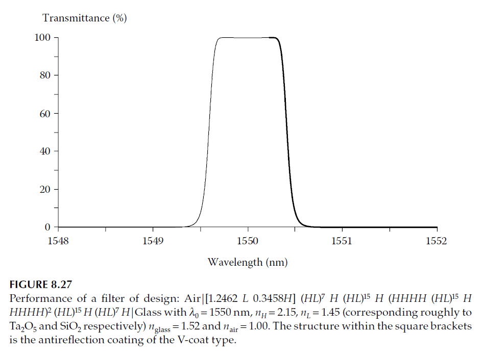
The designs in Figures 8.25 and 8.26 assume identical indices for the incident and emergent media, suitable for embedded filters or those with cemented covers. However, when indices differ, additional matching layers, such as V-coats or multi-layer antireflection coatings, can provide adequate matching. These coatings, while less sensitive to errors than the filter structure, enhance performance and reduce sensitivity to angular incidence (see Figure 8.27).
Advanced Design Techniques
For high-performance filters, manufacturing limitations—such as material constraints and reliance on quarter-wave layers—pose challenges. However, advancements in techniques may relax these constraints. Borrowing methods from microwave design, such as standing wave ratio parameters, enables more flexible and theoretically superior designs.
The standing wave ratio (\(V\)) is defined as:
\[
V = \frac{1 + R}{1 – R} = \frac{E_1 + E_2}{E_1 – E_2}
\]
where \(R\) is the reflectance, and \(E_1\) and \(E_2\) are the electric field amplitudes. For real admittances (\(Y\)) of the system and medium (\(y_0\)), \(V\) simplifies to:
\[
V = \frac{y_0}{Y} \quad \text{or} \quad V = \frac{Y}{y_0}
\]
Microwave structures use iris diaphragm reflectors, replaced in optical filters by thin-film layers. Achieving specific standing wave ratios may require fractional thicknesses or special admittances, often accomplished with symmetrical periods. Manual adjustments, such as replacing single quarter-waves with three-quarter-wave layers, further refine designs.
Example Design
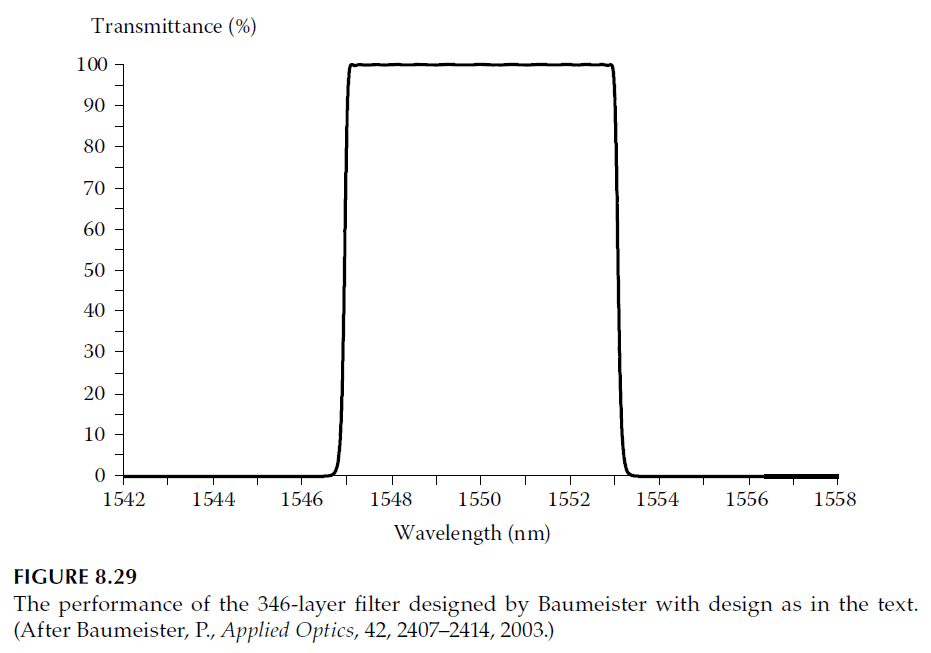
A 13-cavity design using this method, with 346 layers, is:
\[
\text{Air | 0.241L 2.499H 1.241L H (LH)^3 2L (HL)^5 … Glass}
\]
where \(n_{\text{air}} = 1.00\), \(n_H = 2.065\), \(n_L = 1.47\), and \(n_{\text{glass}} = 1.50\).
If designs are constrained to quarter-wave layers of two materials, exact standing wave ratios are unattainable, increasing pass-band ripple. However, these designs remain practical for high-performance filters, balancing theoretical precision and manufacturing feasibility.
1. Effect of Tilting
One notable characteristic of multiple-cavity filter designs is their sensitivity to changes in the angle of incidence. Thelen investigated this aspect, focusing on designs involving symmetrical periods with quarter-waves of alternating high and low refractive indices, where the spacers are of the first order. He derived expressions identical to those of Pidgeon and Smith for single-cavity filters. For angular dependence, the filter behaves like a single layer with an effective refractive index given by:
\[
n^* = \sqrt{n_1 n_2} \quad \text{(where \(n_1 > n_2\))},
\]
or
\[
n^* = \sqrt{\frac{n_1^2 + n_2^2}{2}} \quad \text{(where \(n_2 > n_1\))}.
\]
For higher-order filters, these expressions, along with Expressions 8.34 and 8.36, provide a reliable framework for analysis.
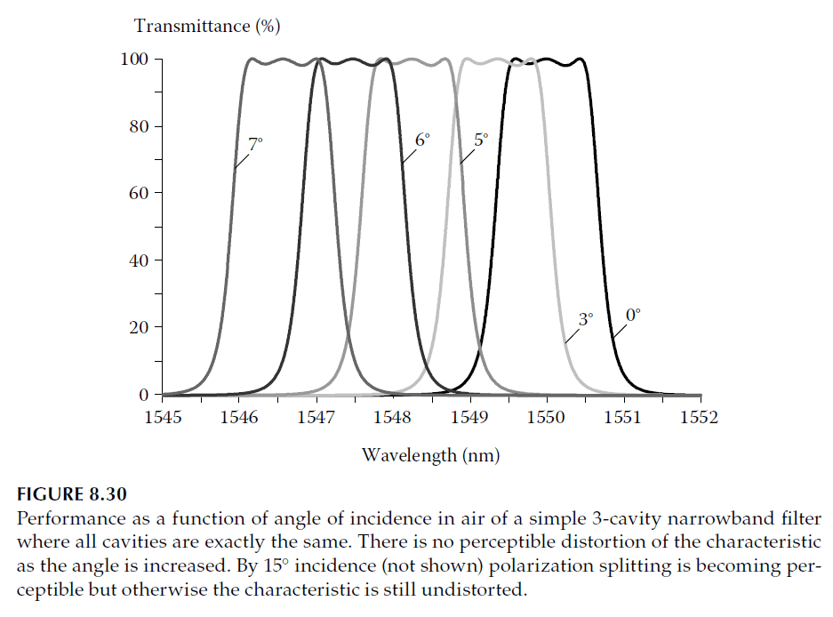
Tilted Performance of Narrowband Filters
Figure 8.30 demonstrates the tilted performance of a simple three-cavity narrowband filter with the following design:
\[
\text{Air | 1.21L 0.38H (HL)}_7 \text{ HHHHHH (LH)}_7 \text{ L (HL)}_7 \text{ HHHHHH (LH)}_7 \text{ L (HL)}_7 \text{ HHHHHH (LH)}_7 \text{| Glass}.
\]
Here, \(n_{\text{air}} = 1.00\), \(n_H = 2.065\), \(n_L = 1.47\), and \(n_{\text{glass}} = 1.50\).
However, complications can arise. Filters like the one shown in Figure 8.27, which use cavities of different orders to achieve excellent ripple performance, experience challenges. These cavities shift at slightly different rates as the angle of incidence changes due to small differences in their effective indices. This detuning degrades the pass-band shape significantly, as shown in Figure 8.31.
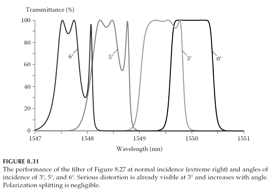
Improving Tilted Performance
To address this degradation, it is necessary to align the effective indices of the cavities more closely. Since high-index cavities generally exhibit higher effective indices, introducing more low-index material into these cavity structures is an effective approach. Trial and error is often the most practical method for achieving the desired balance.
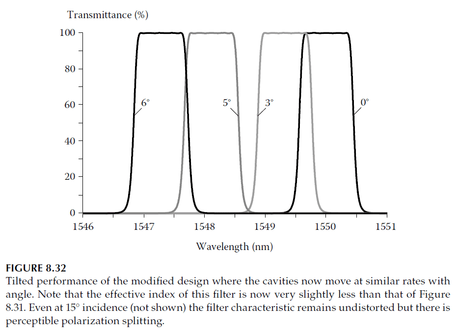
Possible modifications include replacing single low-index quarter-wave layers with three-quarter-wave layers. In this case, changing one or more high-index half-wave layers in the cavity structure to low-index half-wave layers proved effective. The optimized design is as follows:
\[
\text{Air | 1.2676L 0.3379H (HL)}_7 \text{ H (HL)}_{15} \text{ H (HLLH (HL)}_{15} \text{ H HLLH)}_2 \text{(HL)}_{15} \text{ H (HL)}_7 \text{ H | Glass}.
\]
Using the same refractive indices as in Figure 8.27, this design achieves the tilted performance shown in Figure 8.32.
Uniformity Error Compensation
The design shown in Figure 8.29 uses cavities of the same order, resulting in a tilted performance similar to that in Figure 8.32. Filters with reduced sensitivity to tilt angle also exhibit inherent resilience to uniformity errors during deposition.
For narrowband filters, deposition thickness monitoring is often direct, meaning it is performed on an actual filter being produced. This approach allows for error compensation critical to successful narrowband filter production. However, thickness variations can occur outside the monitoring area. Such variations are sometimes intentional, as in telecom filter production, where a single large filter disk is diced into smaller filters post-deposition. Variations in thickness yield filters tuned to different channel wavelengths.
Ensuring uniform thickness across high- and low-index films is challenging, as discrepancies can mimic the effects of tilting. Filters insensitive to changes in tilt angle also exhibit greater tolerance to relative uniformity errors, improving the yield of usable components.
2. Losses in Multiple-Cavity Filters
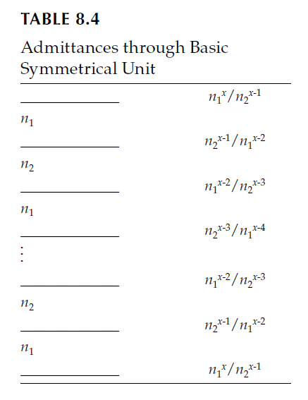
The losses in multiple-cavity filters can be estimated similarly to those in Fabry–Perot filters. While there are countless design possibilities, a completely general approach would be highly complex. To simplify, we start by assuming that the basic symmetrical unit is perfectly matched at both ends. The admittance scheme through the basic unit is then as shown in Table 8.4.
Using the same principles as the single-cavity filter, we can write:
\[
\Sigma A = \beta_1 \left( \frac{n_1}{n_2} – 1 \right) + \beta_2 \left( \frac{n_2}{n_1} – 1 \right) + \ldots
\]
This expression accounts for the summation of losses (\(\Sigma A\)) across all layers, with alternating terms dependent on the indices of refraction (\(n_1\) and \(n_2\)) of the high- and low-index materials. Each term represents the loss contribution of a layer in the structure.
Quarter-Wave Layer Assumptions
As the layers are quarter-waves, the phase shifts (\(\beta_1\) and \(\beta_2\)) can be expressed as:
\[
\beta_1 = \frac{\pi}{n_1 k_1} \quad \text{and} \quad \beta_2 = \frac{\pi}{n_2 k_2},
\]
where \(k_1\) and \(k_2\) are constants related to the physical properties of the layers. Substituting these values into the loss equation allows us to evaluate the total losses for various designs.
High- and Low-Index Cavities
The calculation can be divided into two cases based on whether the cavity layers are of high or low refractive index:
1. High-Index Cavities: These layers exhibit higher \(\beta\) values due to their greater refractive index. Losses tend to accumulate more rapidly in these layers.
2. Low-Index Cavities: These layers contribute less to the total loss because of their lower refractive index, leading to smaller \(\beta\) values.
The balance of high- and low-index layers in a multiple-cavity filter influences its total loss profile. Proper design ensures that the losses are minimized while maintaining the desired filter performance.
Inverse Symmetry in Loss Expressions
Each term in the loss equation appears in pairs, where the second expression of each pair is the inverse of the first. This symmetry simplifies the analysis, as the losses for high- and low-index layers can be combined into a single unified expression.
2.1 Case I: High-Index Cavities
In this case, we replace \(n_1\) with \(n_H\) (high refractive index), \(k_1\) with \(k_H\), \(n_2\) with \(n_L\) (low refractive index), and \(k_2\) with \(k_L\). Neglecting terms proportional to \((n_L / n_H)^x\), as these are much smaller than unity, the absorption loss (\(A\)) for a single symmetrical unit becomes:
\[
A = \pi k_H n_H \left(1 – \frac{n_L^2}{n_H^2}\right) + \pi k_L n_L \left(1 – \frac{n_L^2}{n_H^2}\right),
\]
which simplifies to:
\[
A = \pi \left[k_H n_H + k_L n_L\right] \left(1 – \frac{n_L^2}{n_H^2}\right).
\]
From Expression 8.60 (with \(m = 1\)), the bandwidth is given by:
\[
\Delta \lambda_B = \frac{\lambda_0}{\pi} \frac{n_H – n_L}{n_H n_L} \left(\frac{n_L}{n_H}\right)^x,
\]
which allows us to rewrite the absorption loss as:
\[
A = \frac{\Delta \lambda_B}{\lambda_0} \cdot \frac{4 \pi}{n_H n_L} \left(k_H n_H + k_L n_L\right).
\]
This represents the loss for one basic symmetrical unit. If additional symmetrical units are added, each contributes an equal loss.
Total Loss Across the Filter
In addition to the symmetrical units, matching stacks at both ends of the filter contribute to the total loss. A reasonable assumption is that the loss from the matching stacks equals the loss of one symmetrical unit. The total number of symmetrical units, denoted as \(q\), equals the number of cavities in the filter (e.g., \(q = 2\) for a two-cavity filter). Assuming reflectance (\(R\)) is negligible (\(R = 0\)), the total absorption loss is:
\[
A = q \cdot \pi \left(k_H n_H + k_L n_L\right) \left(1 – \frac{n_L^2}{n_H^2}\right),
\]
or, substituting for bandwidth:
\[
A = q \cdot \frac{\Delta \lambda_B}{\lambda_0} \cdot \frac{4 \pi}{n_H n_L} \left(k_H n_H + k_L n_L\right).
\]
Final Expressions for Total Loss
The loss, considering \(q\) cavities, is expressed as:
1. In terms of refractive indices and absorption coefficients:
\[
A = q \cdot \pi \left[k_H n_H + k_L n_L\right] \left(1 – \frac{n_L^2}{n_H^2}\right).
\]
2. In terms of bandwidth and central wavelength:
\[
A = q \cdot \frac{\Delta \lambda_B}{\lambda_0} \cdot \frac{4 \pi}{n_H n_L} \left(k_H n_H + k_L n_L\right).
\]
These equations provide a practical way to estimate the absorption losses in multiple-cavity filters.
2.2 Case II: Low-Index Cavities
For low-index cavities, the absorption loss (\(A\)) is calculated in a similar manner as for high-index cavities. The result is:
\[
A = q \cdot \pi \left[\frac{n_H}{n_L} \cdot k_L n_L^2 + \frac{n_L}{n_H} \cdot k_H n_H^2 \right] \left(1 – \frac{n_L^2}{n_H^2}\right),
\]
or equivalently:
\[
A = q \cdot \frac{\Delta \lambda_B}{\lambda_0} \cdot 4 \pi \left[k_L \frac{n_H}{n_L} + k_H \frac{n_L}{n_H}\right],
\]
where:
– \(q\): Number of cavities in the filter,
– \(\Delta \lambda_B\): Bandwidth,
– \(\lambda_0\): Central wavelength,
– \(n_H\), \(n_L\): High and low refractive indices, respectively,
– \(k_H\), \(k_L\): Absorption coefficients for high- and low-index materials.
Comparison with Single-Cavity Filters
Expressions 8.66 (from the high-index cavity case) and 8.68 (for the low-index cavity case) show that the absorption loss in multiple-cavity filters is approximately \(q\) times the loss of single-cavity filters with the same half-width. This result is intuitive, as adding more cavities increases the total absorption proportionally.
3. Further Information
The examples of multiple-cavity filters discussed so far have focused on the visible and infrared regions, but these filters can be designed for any part of the spectrum where suitable thin-film materials are available. A comprehensive account of filters for the visible and ultraviolet regions is provided by Barr, which remains relevant to this day.
Ultraviolet Filters
Nielson and Ring described all-dielectric filters, including single-cavity and multiple-cavity types, for the near ultraviolet region. They utilized combinations of:
1. Cryolite and Lead Fluoride: Suitable for the wavelength range of 250–320 nm.
2. Cryolite and Antimony Trioxide: Effective for the range of 320–400 nm.
The key challenge in designing ultraviolet filters lies in the relatively small difference between the high and low refractive indices of the materials. This necessitates the use of more layers to achieve the same level of rejection as filters designed for the visible or infrared spectrum. For instance, Nielson and Ring’s filters included basic units of 17 or 19 layers, resulting in complete double half-wave (DHW) filters with 31 or 39 layers, respectively.
Extreme Ultraviolet Filters
Malherbe described a filter for a wavelength of 205.5 nm using lanthanum fluoride and magnesium fluoride. This filter incorporated a high-index first-order cavity, with the basic unit containing 51 layers. The complete design was as follows:
\[
(\text{HL})_{12} \, \text{H} \, (\text{LH})_{25} \, \text{H} \, (\text{LH})_{12}
\]
This structure comprised a total of 99 layers and achieved a measured bandwidth of 2.5 nm.
Summary
While the fundamental principles of designing multiple-cavity filters remain consistent across different spectral regions, the choice of materials and the number of layers depend heavily on the refractive index contrast available for the specific region. Advances in thin-film deposition techniques continue to expand the applicability of such filters across the ultraviolet, visible, and infrared spectrums.