The transmission curve of the basic all-dielectric single-cavity, or Fabry–Perot, filter is not ideal. It can be shown that half of the energy transmitted in any order lies outside the half-width (assuming an even distribution of energy with frequency in the incident beam).
A more rectangular curve would significantly improve performance. Furthermore, the maximum rejection of the single-cavity filter is constrained by the half-width and the order. Broader filters tend to have poor rejection and a less satisfactory shape.
When tuned electric circuits are coupled, the resultant response curve becomes more rectangular, with greater rejection outside the pass band compared to a single tuned circuit. A similar result is achieved with single-cavity filters. By placing two or more such filters in series, the resultant curve attains a much more desirable shape. These filters may be metal–dielectric or all-dielectric, with the basic structure:
| reflector | half-wave cavity | reflector | half-wave cavity | reflector |
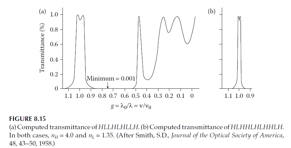
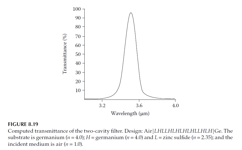
The outer reflectors are typically weaker than the central one. This structure has been referred to by various names, such as double half-wave (DHW) filter, double cavity filter, or two-cavity filter. Examples of all-dielectric two-cavity filters are shown in Figure 8.15.
Such filters were developed by A. F. Turner and colleagues at Bausch and Lomb in the early 1950s, with results published as quarterly reports in the Fort Belvoir Contract Series (1950–1968). Early designs included three-cavity (triple half-wave) filters, termed WADIs (wide-band all-dielectric interference filters), while two-cavity (double half-wave) filters appeared later and were routine by 1957, initially termed TADIs.
The Fort Belvoir reports illustrate the advanced work at Bausch and Lomb, including the use of equivalent admittance for WADI and edge filter design, along with multilayer antireflection coatings. The first comprehensive archival theory of multiple half-wave filters was provided by Smith, whose method is discussed here.
In classic single-cavity filters, reflecting stacks have nearly constant reflectance over the pass band. While phase change dispersion can reduce bandwidth, it does not significantly alter the pass band shape. Smith proposed using reflectors with rapidly varying reflectance to improve shape. The essential transmittance expression, derived in Section 3.7 (assuming β = 0, or no absorption in the cavity layer), is given by Equation 3.19:
\[
T = \frac{\tau_a \tau_b}{1 – \rho_a \rho_b + 4\sqrt{\rho_a \rho_b} \sin^2 \frac{\phi_a + \phi_b + \delta}{2}}
\]
High transmission occurs when the reflectances on either side of the spacer layer are equal, and the phase condition is met:
\[
\phi_a + \phi_b + \delta = m\pi
\]
Here, symbols retain their meanings as defined in Figure 3.8. Smith emphasized low reflectance near the peak wavelength to minimize absorption effects, limiting bandwidth by increasing reflectance disparity at wavelengths slightly removed from the peak (illustrated in Figure 8.16).
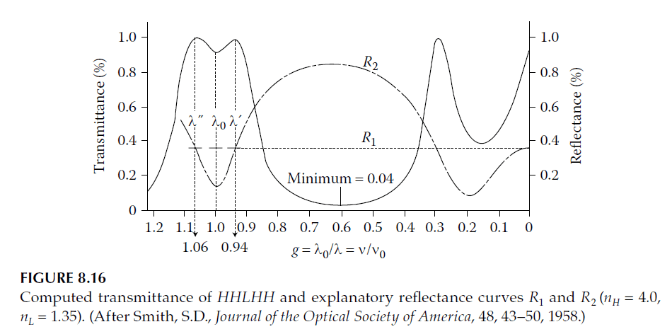
The simplest two-cavity filter structure, HHLHH (where HH represents cavities and L a coupling layer), demonstrates these principles. Figure 8.16 shows a steep-sided pass band with twin peaks close together, resembling an ideal rectangle more than a single-cavity filter.
Smith’s transmittance formula for a filter can be written as:
\[
T(\lambda) = \frac{T_0(\lambda)}{1 + F(\lambda) \sin^2 \left(\frac{\phi_1 + \phi_2 – \delta}{2}\right)}
\]
Where:
\[
T_0(\lambda) = \frac{(1 – R_1)(1 – R_2)}{(1 – \sqrt{R_1 R_2})^2}
\]
\[
F(\lambda) = \frac{4 \sqrt{R_1 R_2}}{(1 – \sqrt{R_1 R_2})^2}
\]
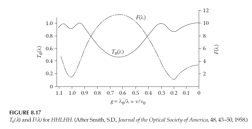
These quantities depend on \(R_2\), which varies with wavelength as shown in Figure 8.17. High transmittance at the peak is achieved with low \(F(\lambda)\), reducing absorption sensitivity.
The characteristic double-peaked shape arises when \(R_1\) and \(R_2\) intersect at two points. Alternative designs involve single peaks (if intersecting once) or reduced transmittance (if no intersection occurs). Shallow troughs between peaks require close \(R_1\) and \(R_2\) values at \(\lambda_0\).
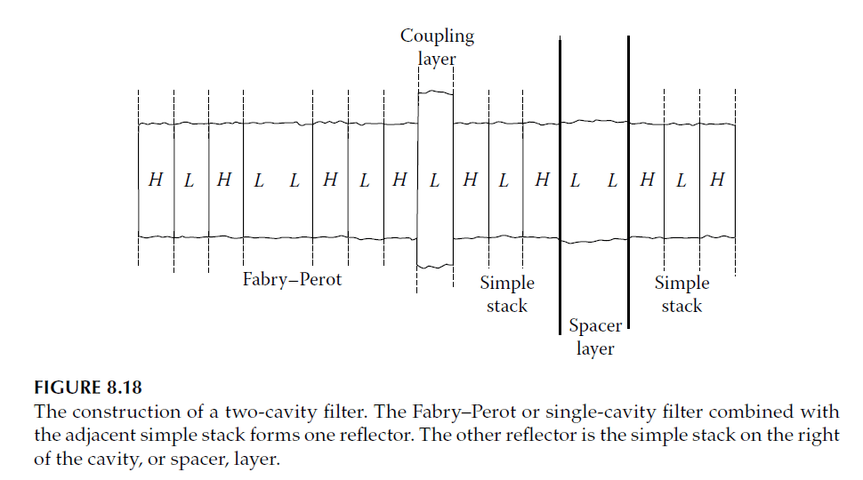
More complex filters involve designing reflectors where one side maintains constant reflectance, and the other varies. This approach produces single- or double-peaked transmission curves, as illustrated in Figure 8.18.
The substrate also influences reflectance and must be incorporated into designs. For instance, filters deposited on germanium substrates using zinc sulfide and germanium layers require adjustments for balance, resulting in configurations like:
\[
\text{Ge | LH LL HLH L HLH LL HLH | air}
\]
Eliminating absentee half-wave layers confirms high transmittance, as the structure reduces to:
\[
\text{Ge | L | air}
\]
Knittl applied a multiple-beam summation method to design two-cavity filters, yielding expressions similar to Smith’s but simpler to manipulate.
Multiple-cavity filters extend beyond two-cavity designs, including WADIs and three-cavity (THW) filters for broader bandwidths and steeper sides. Advanced methods, such as Thelen’s design techniques, are required for further complexity.
Thelen’s Method of Analysis
We have yet to develop an efficient method for calculating the bandwidth of two- and three-cavity filters. The current design method ensures high transmittance in the pass band and steep-sided transmission curves, but determining the bandwidth often requires trial and error to achieve a prescribed value. Although the formula for transmittance:
\[
T = \frac{T_0}{1 + F \sin^2\delta}
\]
can be used, it is labor-intensive as the phases of the reflectances must be included in \(\delta\). While this formula provides insights into the basic properties of multiple-cavity filters, a systematic design method using the concept of equivalent admittance, as proposed by Thelen, is far more practical.
As explained in previous tutorials, any symmetrical thin-film assembly can be replaced with a single layer characterized by an equivalent admittance and optical thickness, both varying with wavelength. Thelen applied this concept to develop a systematic design method that predicts all performance features of filters, including bandwidth. This approach divides the multiple-cavity filter into symmetrical periods, which are analyzed using their equivalent admittances. For example, consider the design:
\[
\text{Ge | LH LL HLH L HLH LL HLH | air}
\]
This can be rearranged as:
\[
\text{Ge | LHL LHLHLHLHL LHLH | air}
\]
Here, the central section (\(LHLHLHLHL\)) is symmetrical and can be replaced by a single layer with alternating high-reflectance zones (imaginary admittance) and pass zones (real admittance). The symmetrical section must be matched to the substrate and surrounding air, achieved by adding matching layers. These layers, all of quarter-wave optical thickness, ensure proper matching.
One significant advantage of this method is the ability to repeat the central section multiple times to steepen the edges of the pass band and enhance rejection without significantly altering the bandwidth.
Predicting Bandwidth
Thelen provided formulae for calculating the bandwidth of the basic sections. Using these, we represent the basic period as:
\[
HmLHLHLH…LHm \quad \text{or} \quad LmHLHLHL…HLm
\]
where there are \(2x + 1\) layers (\(x + 1\) of one refractive index and \(x\) of the other) and \(m\) is the order number. Following Seeley’s [4] approach, the characteristic matrix for a quarter-wave layer near its design wavelength is:
\[
\begin{bmatrix}
0 & -i/n \\
-in & 0
\end{bmatrix}
\]
where \(\epsilon = (\pi/2)(g – 1)\), \(g = \lambda_0 / \lambda\), and \(n\) represents the refractive index. For \(m\) odd (\(m = 2q + 1\)), the matrix for \(Hm\) or \(Lm\) becomes:
\[
\begin{bmatrix}
(-1)^q & -i\epsilon/n \\
-i\epsilon n & (-1)^q
\end{bmatrix}
\]
The matrix product for the symmetrical period with \(2x – 1\) layers is:
\[
\mathbf{M} =
\begin{bmatrix}
M_{11} & iM_{12} \\
iM_{21} & M_{22}
\end{bmatrix}
\]
where:
\[
M_{11} = M_{22} = (-1)^x \left[1 + \frac{\epsilon^2}{2} \left(\frac{n_1}{n_2}\right)^x\right]
\]
\[
M_{12} = M_{21} = (-1)^{x-1} \frac{\epsilon}{n_1^2/n_2^x}
\]
To define the edges of the pass band, Thelen set \(M_{11} = 1\), leading to:
\[
\epsilon \approx \frac{\left(\frac{n_1}{n_2}\right)^x}{m}
\]
The bandwidth \(\Delta \lambda_B\) is then:
\[
\Delta \lambda_B = \frac{\lambda_0}{\pi} \frac{n_H – n_L}{n_H n_L} \left(\frac{n_L}{n_H}\right)^x
\]
This formula applies to both even and odd \(m\).
Design and Matching Layers
Matching the equivalent admittance to the substrate and air requires adding quarter-wave layers with alternating indices (\(n_1\), \(n_2\)) to the symmetrical period. For example, the equivalent admittance of \(LHLHLHLHL\) is:
\[
E = \frac{n_H^5}{n_L^4}
\]
Adding \(LHLH\) transforms the admittance into a perfect match for germanium:
\[
E = \frac{n_L^4}{n_H^4}
\]
Similarly, the matching layers on the air side (\(HLH\)) provide a good match for air, given that zinc sulfide is a good antireflection coating for germanium.
Performance Limitations
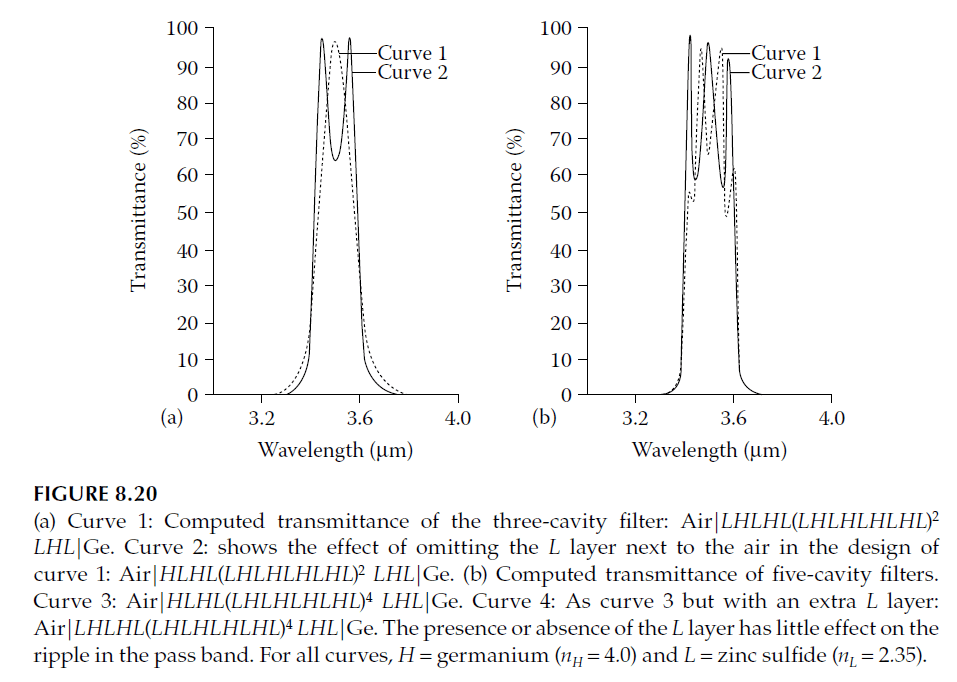
Adding symmetrical periods to the central section narrows fringe widths. If the fringe width becomes narrower than the filter bandwidth, pronounced ripples appear in the pass band, as illustrated in Figure 8.20. While acceptable for three-cavity designs with an additional \(L\) layer, five-cavity designs often become unusable.
Practical Design Considerations
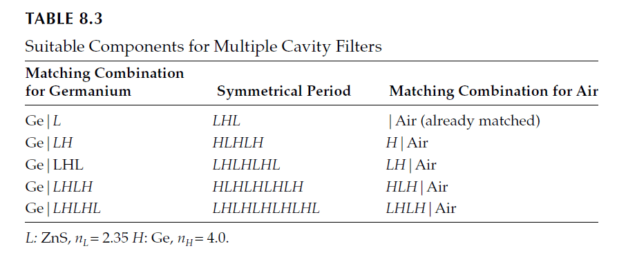
The choice of materials and the number of layers in the central section can be tested using equivalent admittance calculations. Table 8.3 provides combinations for up to 11 layers in the center section.
For higher-order filters, matching layers may include half-wave sections to ensure uniform cavity order. For instance, the design:
\[
\text{Ge | HHHLHLHLHLHHH | air}
\]
can be matched with either \(LHLH\) or \(LHLHHH\), depending on whether uniform cavity order is required.
Final Checks
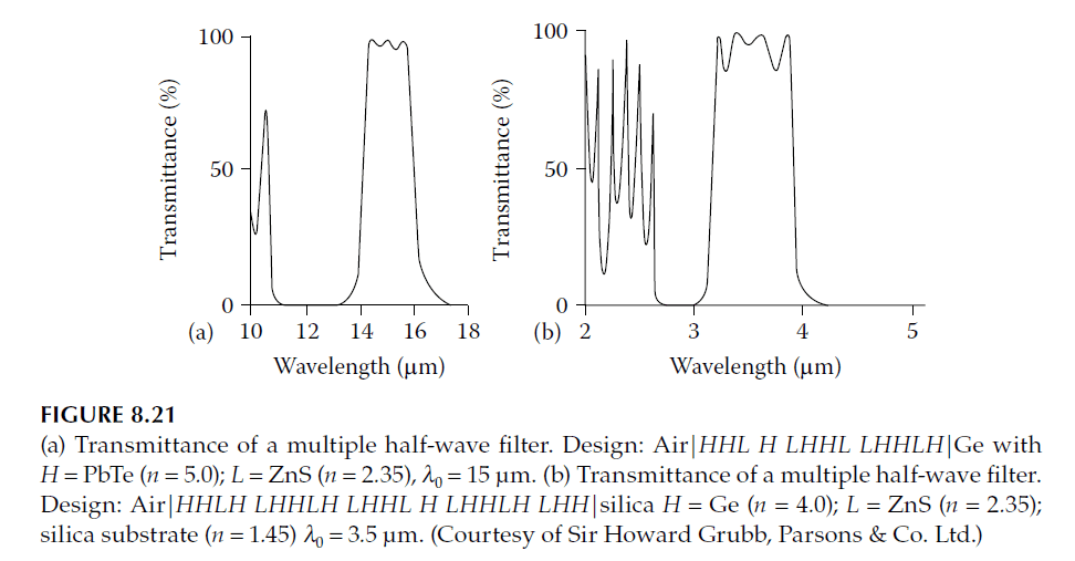
While this method provides systematic guidelines, accurate computations should verify the design before manufacturing. Estimating manufacturing tolerances ensures the achievable performance aligns with process capabilities. Figure 8.21 shows examples of typical multiple-cavity filters.