As with other thin-film assemblies, the performance of the all-dielectric single-cavity filter varies with the angle of incidence. This is particularly important when considering factors like the allowable focal ratio of the beam passing through the filter or the maximum tilt angle in an application. Interestingly, this variation can also be beneficial, as it allows for tuning filters that might otherwise be slightly off the desired wavelength—easing the stringent production tolerances.
The effect of tilting has been studied extensively by researchers such as Dufour and Herpin, Lissberger, Lissberger and Wilcock, and Pidgeon and Smith. Here, we adopt the approach of Pidgeon and Smith due to its suitability.
1. Simple Tilts in Collimated Light
The phase thickness of a thin film at an oblique incidence is given by:
\[
\delta = \frac{2\pi nd \cos \vartheta}{\lambda}
\]
This represents an apparent optical thickness of \( nd \cos \vartheta \), which decreases with the tilt angle, shifting the filter’s pass band to shorter wavelengths.
For an ideal single-cavity filter with a cavity layer of refractive index \( n^* \), where the reflectors have a constant phase shift of 0 or \( \pi \), the peak wavelength in the \( m \)-th order is:
\[
\lambda = \frac{2n^* d \cos \vartheta}{m}
\]
where \( \lambda \) is the tilted peak wavelength, and \( \lambda_0 \) is the peak at normal incidence. Replacing \( \lambda_0 / \lambda \) with \( g \), and writing \( g = 1 + \Delta g \), we find:
\[
1 + \Delta g = \frac{1}{\cos \vartheta}
\]
Thus:
\[
\Delta g = 1 – \cos \vartheta
\]
For an incident angle \( \vartheta_0 \) in air:
\[
\vartheta = \arcsin\left(\frac{\sin \vartheta_0}{n^*}\right)
\]
and \( \Delta g \) becomes a function of \( \vartheta_0 \) and \( n^* \). For small angles of incidence:
\[
\Delta g = \Delta \nu / \nu_0 = \Delta \lambda / \lambda_0 = \frac{n^{*2} \vartheta_0^2}{2}
\]
This equation shows that higher cavity indices \( n^* \) make the filter less sensitive to tilt.
In real filters, tilting also affects the reflectors. However, it has been shown by Pidgeon and Smith [15] that the shift closely matches that of an ideal filter with an “effective index” \( n^* \), typically between the high and low refractive indices of the layers in the filter. This concept holds for tilt angles up to 20°–30° or more, depending on the materials.
Calculating Effective Index
The peak wavelength is given by:
\[
\sin^2\left(\frac{2\pi nd \cos \vartheta}{\lambda}\right) – \phi = 0
\]
At normal incidence (\( \vartheta = 0 \)):
\[
\sin^2\left(\frac{2\pi nd}{\lambda_0}\right) – \phi = 0
\]
Thus:
\[
\frac{2\pi nd}{\lambda_0} = m\pi, \quad m = 0, 1, 2, \dots
\]
For small perturbations (\( \Delta g \)) around the normal incidence peak position:
\[
\sin^2\left[\frac{2\pi nd}{\lambda_0} \left(1 + \Delta g\right) \cos \vartheta – \phi\right] = 0
\]
Replacing \( \cos \vartheta \) with \( 1 – \vartheta_0^2 / (2n^2) \) and expanding, we find:
\[
m\pi \Delta g – m\pi \frac{\vartheta_0^2}{2n^2} – \Delta \phi = 0
\]
Phase Shift Adjustments
From Equations 8.20 and 8.21:
\[
\epsilon = \frac{\pi}{2}\left(g – 1\right)
\]
where \( g = \lambda_0 / \lambda \). This applies separately for high-index and low-index cavities. Substituting for \( \epsilon \) in terms of tilt parameters:
\[
\epsilon = \frac{\pi \vartheta_0^2}{4n^2}
\]
The phase shift \( \phi \) is adjusted based on the indices and tilt angle. The resulting filter performance depends on these corrections, allowing better prediction and tuning under tilted conditions.
For further clarity and application-specific derivations, each case (high-index and low-index cavities) must be treated separately.
2. Case I: High-Index Cavities
For high-index cavities, using Equation 8.20 and inserting \( n_H \) for \( \eta_0 \), the phase shift \( \Delta \phi \) becomes:
\[
\Delta \phi = \frac{\epsilon_H – \epsilon_L}{\epsilon_H + \epsilon_L} \approx \frac{n_H^2 – n_L^2}{n_H^2 + n_L^2}
\]
where \( \epsilon_H \) and \( \epsilon_L \) are perturbation terms for high- and low-index layers, respectively. Incorporating the terms for angle-related changes, we get:
\[
\Delta \phi = \frac{n_H^2 – n_L^2}{n_H^2 + n_L^2} – \frac{\pi}{2} \cdot \frac{\vartheta_0^2}{n_H^2}.
\]
For the relative wavelength shift \( \Delta g \), we have:
\[
\Delta g = \frac{\pi \vartheta_0^2}{2} \cdot \frac{n_H^2 – n_L^2}{n_H^2 n_L^2}.
\]
Substituting these into Equation 8.33 for peak shift:
\[
m\pi \Delta g – \frac{m\pi \vartheta_0^2}{2 n_H^2} – \Delta \phi = 0.
\]
After simplification, this gives:
\[
\Delta g = \frac{\vartheta_0^2}{2} \left( \frac{n_H^2 – n_L^2}{n_H^2 n_L^2} – \frac{1}{m n_H^2} \right).
\]
Effective Index for High-Index Cavities
Comparing the above expression for \( \Delta g \) with Equation 8.29:
\[
\Delta g = \frac{\vartheta_0^2}{2 n^{*2}},
\]
we can solve for the effective index \( n^* \) as:
\[
n^* = \left[ \frac{n_H^2 – n_L^2}{n_H^2 n_L^2} – \frac{1}{m n_H^2} \right]^{-1/2}.
\]
For large \( m \), the term \( 1 / (m n_H^2) \) becomes negligible, and \( n^* \) approaches:
\[
n^* = \sqrt{\frac{n_H^2 + n_L^2}{2}},
\]
which is consistent with Pidgeon and Smith’s result for first-order filters.
First-Order Filter Approximation
For first-order filters (\( m = 1 \)):
\[
n^* = \sqrt{n_H n_L}.
\]
As \( m \to \infty \), \( n^* \to n_H \), reflecting the dominance of the high-index material in determining the optical response. This shows the sensitivity of the filter to angular tilts is determined by the balance between \( n_H \) and \( n_L \).
3. Case II: Low-Index Cavities
The analysis for low-index cavities follows the same method as for high-index cavities, except that Equation 8.22 is used, and \( n \) in Equation 8.33 becomes \( n_L \). The effective index \( n^* \) is given by:
\[
n^* = \left[ \frac{m – 1}{m} n_L^2 + \frac{1}{m} n_H^2 \right]^{1/2}.
\]
For **first-order filters** (\( m = 1 \)):
\[
n^* = \left[ \frac{n_L^2 + n_H^2}{2} \right]^{1/2}.
\]
As \( m \to \infty \), \( n^* \to n_L \), as expected for a low-index cavity. This result is consistent with Pidgeon and Smith’s analysis.
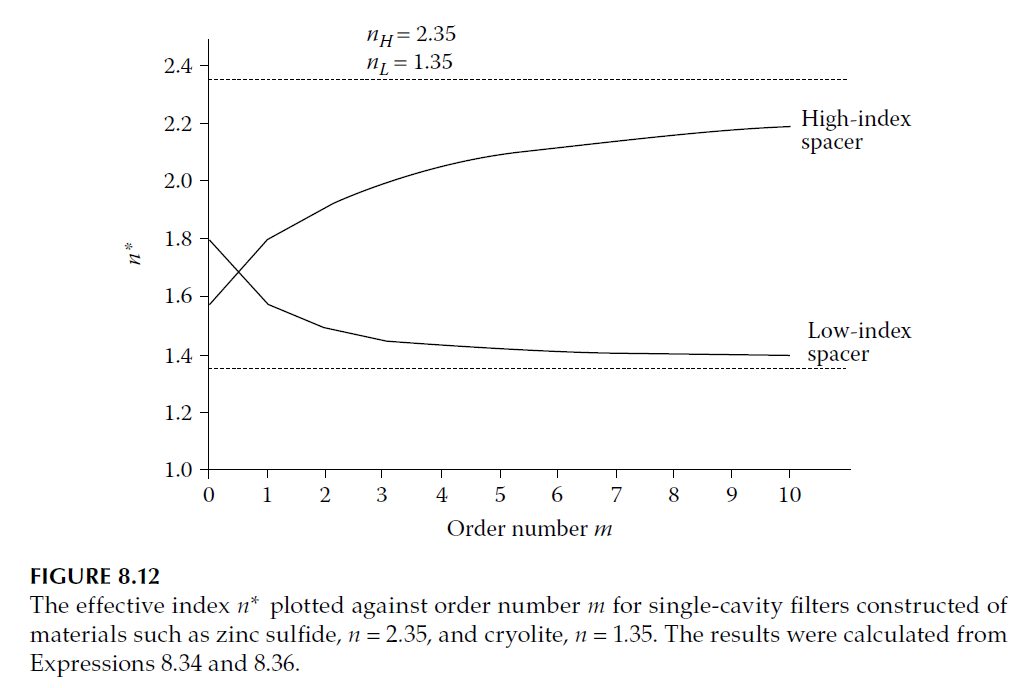
Variation of Effective Index \( n^* \) with Order
Typical curves showing how \( n^* \) varies with the order number for both low- and high-index cavities are presented in Figure 8.12. For low-index cavities, the effective index approaches \( n_L \) as the cavity order increases, while for high-index cavities, it approaches \( n_H \).
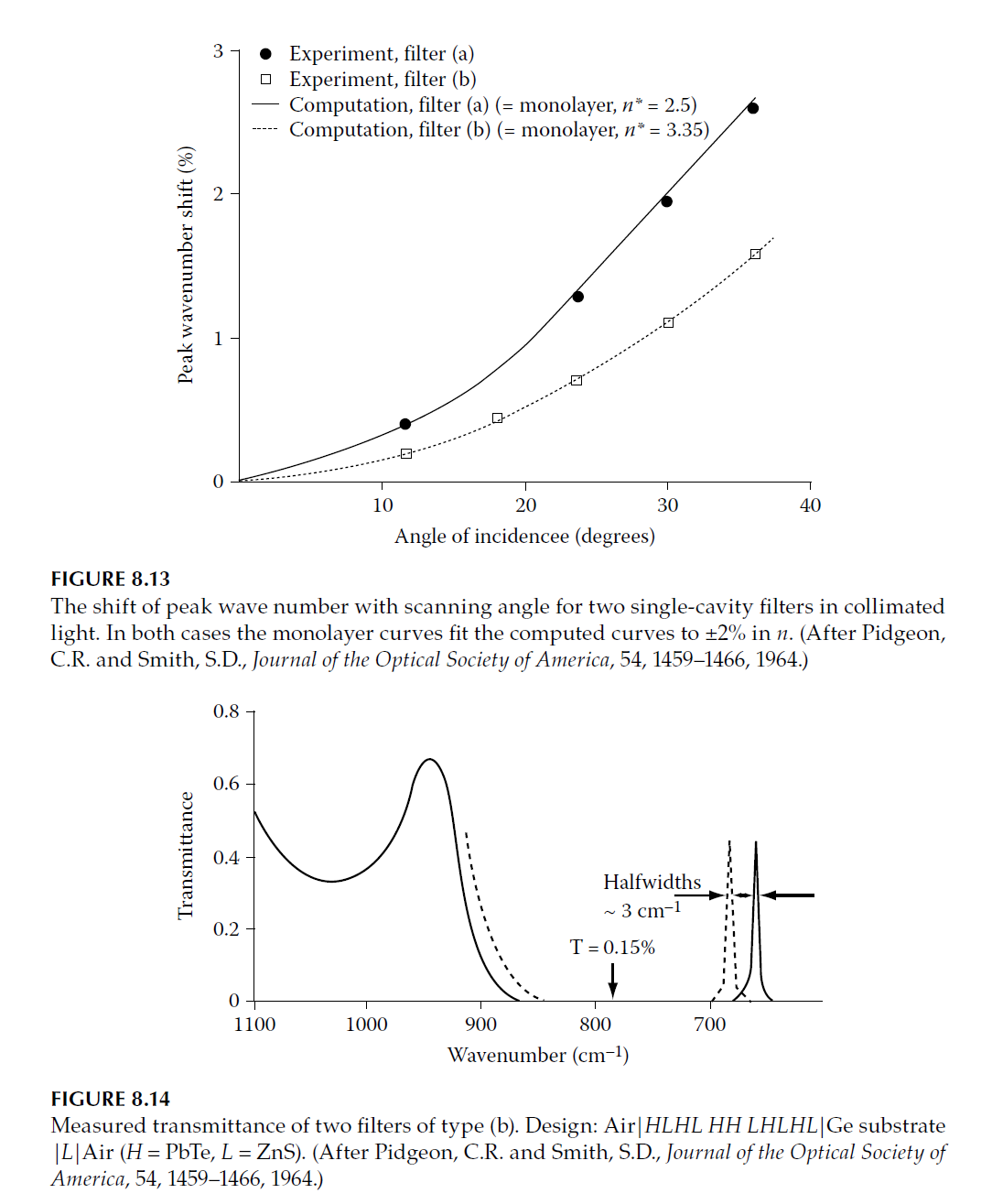
Experimental Measurements by Pidgeon and Smith
Pidgeon and Smith conducted experimental studies on narrowband filters for the infrared. The designs were:
– (a) \( L|Ge|LHLH LL HLH|Air \)
– (b) \( L|Ge|LHLHL HH LHLH|Air \)
Here:
– \( H \): Quarter-wave thickness of lead telluride.
– \( L \): Quarter-wave thickness of zinc sulfide.
– Peak wavelength: Approximately \( 15 \, \mu\text{m} \).
Calculation of Shift
Shifts in peak wavelength were calculated using the approximate method (with \( n^* \)) and the full matrix method (without approximations). The results matched closely, with an accuracy of ±2% in \( n^* \) for angles of incidence up to \( 40^\circ \). Experimental data showed excellent agreement with theoretical predictions. Results are depicted in Figure 8.13 and Figure 8.14.
Angle of Incidence in a Medium Other than Free Space
If the angle of incidence \( \vartheta_0 \) is in a medium with refractive index \( n_0 \), Equation 8.29 becomes:
\[
\Delta g = \frac{\Delta \nu}{\nu_0} = \frac{\Delta \lambda}{\lambda_0} = \frac{\vartheta_0^2}{2 n_0^2 n^{*2}},
\]
where \( \vartheta_0 \) is measured in radians.
If \( \vartheta_0 \) is in degrees, the equation becomes:
\[
\Delta g = \frac{\Delta \nu}{\nu_0} = \frac{\Delta \lambda}{\lambda_0} = 1.5 \times 10^{-4} \cdot \frac{\vartheta_0^2}{n_0^2 n^{*2}}.
\]
4. Effect of an Incident Cone of Light
The performance of a thin-film filter degrades when the incident light is not perfectly collimated. This section discusses the effect of an incident cone of light on the peak transmission and bandwidth of a narrowband filter. Analyses by Lissberger and Wilcock and Pidgeon and Smith provide the basis for the derivation of these effects.
Shift in Peak Position
When a cone of semiangle \( \Theta \) illuminates the filter, the filter’s peak appears to shift towards shorter wavelengths (or higher wave numbers). The new peak wave number is given by:
\[
\nu_{\text{peak}} = \nu_0 + \frac{\Delta \nu’}{2},
\]
where \( \Delta \nu’ \) is the shift from normal incidence due to the angle of incidence \( \Theta \):
\[
\Delta \nu’ = \nu_0 \frac{\Theta^2}{2n^{*2}}.
\]
Here:
– \( \nu_0 \): Wave number at normal incidence.
– \( n^* \): Effective refractive index of the cavity.
Broadening of Bandwidth
The bandwidth of the filter broadens when illuminated by a cone of light. The effective bandwidth \( W_\Theta \) is given by:
\[
W_\Theta = \sqrt{W_0^2 + (\Delta \nu’)^2},
\]
where \( W_0 \) is the bandwidth at normal incidence.
Reduction in Peak Transmission
The peak transmission decreases due to the angular spread of the incident light. The reduced transmission is expressed as:
\[
\hat{T} = \frac{\arctan \left( \frac{\Delta \nu’}{W_0} \right)}{\frac{\Delta \nu’}{W_0}}.
\]
For small values of \( \Delta \nu’ / W_0 \), the transmission can be approximated as:
\[
\hat{T} = 1 – \frac{1}{3} \left( \frac{\Delta \nu’}{W_0} \right)^2.
\]
Analysis of Incident Cone of Light
Assuming the incident light forms a cone with semiangle \( \Theta \), the total transmitted flux is the integral of the transmission function over all angles of incidence. The effective peak position, bandwidth, and transmission can then be derived.
1. Shift in Peak Wavelength:
For a cone of semiangle \( \Theta \), the peak wavelength shift is proportional to the mean of the values at the extreme angles of the cone:
\[
\Delta \nu’ = \nu_0 \frac{\Theta^2}{2n^{*2}}.
\]
2. Broadening of Bandwidth:
The resultant bandwidth is the convolution of the original bandwidth and the angular spread:
\[
W_\Theta = \sqrt{W_0^2 + (\Delta \nu’)^2}.
\]
3. Reduction in Peak Transmission:
The reduction in peak transmission is a function of the angular spread of the light:
\[
\hat{T} = \frac{\arctan \left( \frac{\Delta \nu’}{W_0} \right)}{\frac{\Delta \nu’}{W_0}}.
\]
Oblique Incidence of Conical Light
For an incident cone at an oblique angle \( \chi \), the range of incident angles is \( \chi \pm \Theta \). In this case:
– The new peak position becomes:
\[
\nu_{\text{peak}} = \nu_0 + \frac{\nu_1 + \nu_2}{2},
\]
where \( \nu_1 \) and \( \nu_2 \) correspond to \( \chi – \Theta \) and \( \chi + \Theta \), respectively.
– The bandwidth increases as:
\[
W_\Theta = \sqrt{W_0^2 + (\nu_2 – \nu_1)^2}.
\]
Illustrative Example
For a zinc sulfide and cryolite filter in the visible region:
– Assume a low-index first-order filter with a bandwidth of 1%.
– Effective index: \( n^* = 1.55 \).
– A 10% reduction in peak transmission is acceptable.
1. Tolerance for Cone Semiangle:
Using:
\[
\Delta \nu’ = \nu_0 \frac{\Theta^2}{2n^{*2}},
\]
and requiring \( \Delta \nu’ / W_0 = 0.55 \), the tolerable cone semiangle is approximately \( \Theta = 9.4^\circ \).
2. Peak Shift:
The peak shifts by \( 0.275\% \) towards shorter wavelengths.
3. Oblique Incidence:
At oblique incidence, the tolerable cone angle decreases with increasing tilt.
Practical Considerations
– Optimal Tuning: Filters should be slightly red-shifted during manufacturing to compensate for peak shifts caused by conical illumination.
– Application: The filter’s performance must be optimized for both normal and oblique illumination, considering the tolerable reduction in transmission and broadening of the bandwidth.
5. Sideband Blocking
The all-dielectric filter has a significant limitation: the high-reflectance range of the reflecting coatings is narrow, which restricts the rejection zone of the filter. This limitation can lead to unwanted transmission sidebands, particularly in the longwave and shortwave regions.
Shortwave Sideband Suppression
In the near ultraviolet, visible, and near infrared spectral regions:
– Shortwave sidebands can typically be suppressed using absorption filters with a longwave-pass characteristic.
– These filters are straightforward to apply and are effective at eliminating unwanted shortwave transmissions.
Challenges with Longwave Sidebands
– Longwave sidebands are more difficult to manage:
– They may lie outside the detector’s sensitivity range and thus not require blocking.
– If problematic, they must be addressed with additional measures.
Solutions for Longwave Sidebands
The usual method to eliminate longwave sidebands involves:
1. Adding a metal–dielectric filter:
– Typically a first-order metal–dielectric filter with no longwave sidebands.
– The filter is much broader than the narrowband component to maintain **high peak transmittance**.
2. Integration:
– The metal–dielectric filter can either be:
– Deposited over the basic Fabry–Perot structure.
– Added as a separate component for ease of manufacturing and tuning.
Use of Double Cavity Metal–Dielectric Filters
– Instead of a single cavity filter, a double cavity metal–dielectric filter is often employed.
– Double cavity designs provide better sideband suppression while maintaining high performance.
Transition to Multiple Cavity Filters
The discussion on sideband blocking naturally leads to the next topic: multiple cavity filters, which offer even more precise control over sideband suppression and filter performance. These will be discussed in the following sections.